SIT741 Statistical Data Analysis Assignment Sample

Q1: Car accident dataset (10 points)

Q1.1: How many rows and columns are in the data? Provide the output from your R Studio

Q1.1: What data types are in the data? Use data type selection tree and provide detailed explanation. (2 points for data types, 2 points for explanation)

Q1.3: How many regions are in the data? What time period does the data cover? Provide the output from your R Studio

Q1.4: What do the variables FATAL and SERIOUS represent? What’s the difference between them?

Q2: Tidy Data

Q2.1 Cleaning up columns. You may notice that the road traffic accidents csv file has two rows of heading. This is quite common in data generated by BI reporting tools. Let’s clean up the column names. Use the code below and print out a list of regions in the data set.

Q2.2 Tidying data

a) Now we have a data frame. Answer the following questions for this data frame.

- Does each variable have its own column? (1 point)

- Does each observation have its own row? (1 point)

- Does each value have its own cell? (1 point)

b) Use spreading and/or gathering (or their pivot_wider and pivot_longer new equivalents) to transform the data frame into tidy data. The key is to put data from the same measurement source in a column and to put each observation in a row. Then, answer the following questions.

I. How many spreading (or pivot_wider) operations do you need?

II. How many gathering (or pivot_longer) operations do you need?

III. Explain the steps in detail.

IV. Provide/print the head of the dataset.

c) Are the variables having the expected variable types in R? Clean up the data types and print the head of the dataset.

d) Are there any missing values? Fix the missing data. Justify your actions.

Q3: Fitting Distributions

In this question, we will fit a couple of distributions to the “TOTAL_ACCIDENTS” data.

Q3.1: Fit a Poisson distribution and a negative binomial distribution on TOTAL_ACCIDENTS. You may use functions provided by the package fitdistrplus.

Q3.2: Compare the log-likelihood of two fitted distributions. Which distribution fits the data better? Why?

Q3.3 (Research Question): Try one more distribution. Try to fit all 3 distributions to two different accident types. Combine your results in the table below, analyse and explain the results with a short report.

Q4: Source Weather Data

Above you have processed data for the road accidents of different types in a given region of Victoria. We still need to find local weather data from the same period. You are encouraged to find weather data online.

Besides the NOAA data, you may also use data from the Bureau of Meteorology historical weather observations and statistics. (The NOAA Climate Data might be easier to process, also a full list of weather stations is provided here: https://www.ncei.noaa.gov/pub/data/ghcn/daily/ghcnd-stations.txt )

Answer the following questions:

Q4.1: Which data source do you plan to use? Justify your decision. (4 points)

Q4.2: From the data source identified, download daily temperature and precipitation data for the region during the relevant time period. (Hint: If you download data from NOAA https://www.ncdc.noaa.gov/cdo-web/, you need to request an NOAA web service token for accessing
the data.)

Q4.3: Answer the following questions (Provide the output from your R Studio):

- How many rows are in your local weather data?

- What time period does the data cover?

Q5 Heatwaves, Precipitation and Road Traffic Accidents

The connection between weather and the road traffic accidents is widely reported. In this task, you will try to measure the heatwave and assess its impact on the road accident statistics. Accordingly, you will be using the car_accidents_victoria dataset together with the local weather data.

Q5.1. John Nairn and Robert Fawcett from the Australian Bureau of Meteorology have proposed a measure for the heatwave, called the excess heat factor (EHF). Read the following article and summarise your understanding in terms of the definition of the EHF. https://dx.doi.org/10.3390%2Fijerph120100227

Q5.2: Use the NOAA data to calculate the daily EHF values for the area you chose during the relevant time period. Plot the daily EHF values.

Q6: Model Planning

Careful planning is essential for a successful modelling effort. Please answer the following planning questions.

Q6.1. Model planning:

a) What is the main goal of your model, how it will be used?

b) How it will be relevant to the emergency services demand?

c) Who are the potential users of your model?

Q6.2. Relationship and data:

a) What relationship do you plan to model or what do you want to predict?

b) What is the response variable?

c) What are the predictor variables?

d) Will the variables in your model be routinely collected and made available soon enough for prediction?

e) As you are likely to build your model on historical data, will the data in the future have similar characteristics?

Q6.3. What statistical method(s) will be applied to generate the model? Why?

Q7: Model The Number of Road Traffic Accidents

In this question you will build a model to predict the number of road traffic accidents. You will use the car_accidents_victoria dataset and the weather data. We can start with simple models and gradually makemthem more complex and improve them. For example, you can use the EHF as an additional predictor to augment the model. Let’s denote by Y the road traffic accident variable.

Randomly pick a region from the road traffic accidents data.

Q7.1 Which region do you pick?

Q7.2 Fit a linear model for Y according to your model(s) above. Plot the fitted values and the residuals. Assess the model fit. Is a linear function sufficient for modelling the trend of Y? Support your conclusion with plots.

Q7.3 As we are not interested in the trend itself, relax the linearity assumption by fitting a generalised additive model (GAM). Assess the model fit. Do you see patterns in the residuals indicating insufficient model fit?

Q7.4 Compare the models using the Akaike information criterion (AIC). Report the best-fitted model through coefficient estimates and/or plots.

Q7.5 Analyse the residuals. Do you see any correlation patterns among the residuals?

Q7.6 Does the predictor EHF improve the model fit?

Q7.7 Is EHF a good predictor for road traffic accidents? Can you think of extra weather features that may be more predictive of road traffic accident numbers? Try incorporating your feature into the model and see if it improves the model fit. Use AIC to prove your point.

Q8: Reflection

In the form of a short report answer the following questions (no more than 3 pages for all questions):

Q8.1: We used some historical data to fit regression models. What additional data could be used to improve your model?

Q8.2: Overall, have your analyses answered the objective/question that you set out to answer?

Q8.3: Missing value [10 marks]. If the data had some with missing values, what methods would you use to address this issue? (Provide 1-3 relevant references)

Q8.4. Overfitting [10 marks]. In Q7.4 we used the Akaike information criterion (AIC) to compare the models. How would you tackle the overfitting problem in terms of the number of explanatory variables that you could face in building the model? (Provide 1-3 relevant references)

Solution

Q1. Car Accident Dataset

Q1.1 Dataset description

Figure 1: Dimension of Dataset
(Source: R Studio)

The Dataset contains 1644 Rows and 29 Columns which are generated using the “dim” code.

Q1.2 Data type identification

Figure 2: Type of Dataset
(Source: R Studio)

The Dataset is based on the character datatype which means every data in the dataset contains one byte character.

Figure 3: Selection Tree Code
(Source: R Studio)

The code sets each column of the `car_accidents” dataset and identifies and prints the data type of each column used in this dataset. The type function for The Assignment Helpline determines whether the column is of “numeric”, “character”, “factor” or “date” and returns the type. It has proved to be useful for the identification of the structure of the datasets necessary for further steps of data preprocessing and analysis in the research.

Q1.3 Identification of the regions in dataset

Figure 4: Number of Regions
(Source: R Studio)

In the Dataset, there are a total of 7 regions available which are generated using the given codes.

Figure 5: Date Range
(Source: R Studio)

The Dataset covers the date range between 1st January 2016 to 30th June 2020.

Q1.4 Representation of FATAL and SERIOUS variables

The variables FATAL and SERIOUS are measures of the number of road traffic accidents by area of the world in which they occurred. FATAL shows the total, fatal pedestrian accidents and SERIOUS, indicates the number of severe, but not fatal, injuries. The critical difference lies in the outcome: fatalities refer to loss of lives while serious injuries point towards possible long-term health complications (Jiang et al. 2024). This is particularly important in terms of evaluation of the level of acuity and hence, of resource use in emergency services treatment.

Q2. Tidy Data

Q2.1 Cleaning up columns.

Figure 6: Cleaning up Columns
(Source: R Studio)

The code removes some unwanted characters and spaces from the column names of car accident data which are available in the car_accidents_victoria.csv file data set, In this file there are two rows of headers. The first two rows are read separately, various double underscores are used to generate different names for the columns, and the number ‘0’ is added to certain columns. The column named daily_acccidents is then taken from the cleaned dataset after omitting the first two rows of the Excel file and the column headers are given standard names for further use. This makes certain data manipulation to be correct and makes subsequent modelling to be clear.

Q2.2 Tidying data

a

Figure 7: Column Identification
(Source: R Studio)

The code then demonstrates whether each variable in the daily_accidents dataset is properly indexed in its column by using the is.atomic function. The output reproduced this with the value of `TRUE’ signifying that the data was well formatted for analysis.

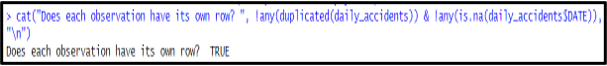
Figure 7: Row Identification
(Source: R Studio)

The code guarantees each observation in the daily_accidents has its row by way of checking to ensure no rows are repeated in the dataset while also ensuring the DATE column does not hold any missing values. The TRUE output as shown below also accredits the correct structuring of the data for analysis.

Figure 8: Cell Identification
(Source: R Studio)

It also confirms that each value in the daily_accidents dataset has its row by using is.na() to test that no value in this dataset is missing. To output FALSE, there is likely an information quality problem which is always common with data, that makes them improper for further analysis.

b

i)

Figure 9: Pivot Wider
(Source: R Studio)

A single `pivot_wider` transformation process is required to keep reshaping the dataset by widening different types of accidents, namely the accident type (FATAL, SERIOUS), which has to be categorized distinctly for every observation.

ii)

Figure 10; Pivot Longer
(Source: R Studio)

To merge multiple region-based columns into a single spread column while ensuring that all are under one variable to return the data to their tidy shape a double `pivot_longer` is needed.

iii)

The code begins with the `pivot_longer` function to transform multiple region-specific accident columns into one single column called `Region` which subsumes the types of accidents (FATAL, SERIOUS) under the column title `Accident_Type`. The `names_pattern` argument inputs the substring `Region` and `Accident_Type` out of column names because their matching is assumed to be most precise in the usage of regular expressions. Then the resulting long-format data is processed using `pivot_wider` and `Accident_Type` values are turned into variables. This extends the row of columns horizontally so that each type of accident is separated by its column, thus simplifying analysis between areas. The last `tidy_data’ format is convenient for the further analysis and modelling phase, visualisation and other statistical techniques (Pereira et al. 2019).

iv)

Figure 11: Head of Data
(Source: R Studio)

The code reshapes the ‘daily_accidents’ dataset so that it has a tidy form. The `long_data’ shows the same accident data as in the previous exercise but this data is in a long format with columns Region, Accident_Type, and their values. The `tidy_data` format then broadens these accident types into individual columns to make a clearer structure for counting accidents within regions over time.

c

Figure 12: Head Data
(Source: R Studio)

The various variables in the dataset might not be initially or automatically read in the expected form, for example, `DATE` may be read as a character `Date`(s), or accident counts as characters. For data type correction, there is a need to transform DATE to Date type while accident columns to numeric form of data. This improves the analysis of the data and also prevents a mistake made during data modelling from going unnoticed.

d

Yes, there are many cases of missing values in the dataset that lead to distortion of results. It is better to use the median or something called forwards filling because trends are weighed in such cases and they do not mislead in case some values are missing.

Q3. Fitting Distribution

Q3.1 Poisson distribution and a negative binomial distribution

Figure 13: Poisson Distribution
(Source: R Studio)

Poisson & Negative binomial distributions are then fitted on the `TOTAL_ACCIDENTS’ variable using the ‘fitdistrplus’ package. It can summarise and plot both models for easy comparison of goodness of distribution fit. This helps in its estimation to know which model best suits the prediction of variation in the accident count.

Q3.2 Comparison of the log-likelihood

Figure 14: LogLikelihood
(Source: R Studio)

The Negative Binomial model again is found to have a better fit with the data as its log-likelihood (-179060.2) is higher than that of Poisson ( -186547.4) while its AIC ( 358124.4) and BIC ( 358141.8) are comparatively lower to that of Poisson. This implies improved data modelling because the uncertainty in measurement is preserved as will be discussed later.

Q3.3 Research Question

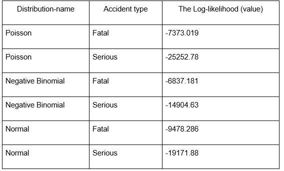
Table 1: Poisson Distribution
(Source: Self-Created)

According to the results, the Negative Binomial distribution has more log-likelihood values for Fatal and Serious types among all the analysed models, which means they are adjusted better than Poisson and Normal distributions. Negative Binomial is more appropriate where the variability of variance is high such as in accident modelling. The Poor fit of Poisson distribution indicates that it is inefficient for capturing the variability of the data, majority while the Moderate fit of the Normal distribution to the current data shows it is imprecise in estimation of count-based accident data. Therefore, the Negative Binomial model is suitable for this dataset in particular because of the effectiveness of its estimation in the case of overdispersion.

Q.4: Source Weather Data

Q.4.1 Data source justification

The historical weather observation data from the Bureau of Meteorology is chosen for its rich and accurate record of the environmental data, which is necessary for estimating the correlation between different weather conditions and traffic crash rates on the roads.

Q.4.2 Downloading dataset

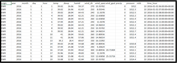
Figure 14: Downloaded Dataset
(Source: EXCEL)

The Dataset is downloaded from the Bureau of Meteorology website.

Q.4.3 Answer the following questions (Provide the output from your R Studio):

Figure 15: Rows Identification
(Source: R Studio)

In the dataset there are 26115 rows are available.

Figure 16: Time Period
(Source: R Studio)

Time period is covered within 1st January 2016 to 30th December 2016.

Q.5: Heatwaves, precipitation and road traffic accidents

Q5.1 Summarization of the understanding

The Excess Heat Factor (EHF) measures heatwave intensity by analysing short-term and long-term heat anomalies. It compares the 30-day average to a three-day mean daily temperature above the 95th percentile. A high EHF indicates a severe heatwave, indicating health and environmental damage.

Q.5.2 Calculate the daily EHF values

Figure 17: EHF Factor
(Source: R Studio)

The graph shows January 2016–January 2017 daily Excess Heat Factor (EHF) data. The highest heat intensity was in April 2016. Summer EHF spikes are more frequent and intense, indicating heat stress. Heatwave severity decreases during cooler seasons.

Q.6: Model planning

Q.6.1 Model planning:

a)

The main goal is to predict road accidents using meteorological data for proactive traffic management and safety planning.

b)

Emergency services can disperse resources and reduce response times by predicting accident hotspots with the model.

c)

Traffic management, emergency services, urban planners, insurance companies, and public safety agencies can use it to improve road safety and resource allocation.

Q.6.2 Relationship and data

a)

Meteorological parameters like temperature, humidity, and EHF are linked to road accidents in different regions by the model. Accident probability and intensity are predicted based on meteorological conditions to aid prevention and resource allocation.

b)

Number of Road Accident will be the Response Variable from the car accident dataset.

c)

Temperature (temp), Humidity (humid), and Excess Heat Factor (EHF) are predictor variable from weather dataset

d)

Meteorological authorities collect and modify temperature, humidity, and EHF in real time to ensure accurate road accident predictions.

e)

In the absence of significant climatic alterations, meteorological patterns and vehicular accident trends are expected to adhere to seasonal fluctuations, rendering the model relevant for future forecasts.

Q.6.3 Application of the statistical model

Linear Regression will be employed for trend analysis, whereas Generalised Additive Models (GAM) will be utilised for non-linear relationships between weather and accident frequency. These methods enable the representation of smooth functions for variables such as temperature and humidity, which may not influence accidents linearly, to elucidate complex interconnections and improve forecasting precision.

Q.7 Model the Number of Road Traffic Accidents

Q.7.1 Region selection

Western Region is selected for the modelling.

Q.7.2 Fitting linear model

Figure 18: Linear Model
(Source: R Studio)

This graph compares the number of accidents in the WESTERN region (blue lines) to the linear model's predictions (red line). Despite increases in accident numbers, the linear model remains constant, failing to capture these oscillations. It appears that a linear model cannot accurately capture road accident trends. Systematic patterns in the residuals plot suggest that a Generalised Additive Model (GAM) might be better at capturing non-linear interactions. By showing that complex models improve predictions, this influences research.

Q.7.3 Fitting a generalised additive model

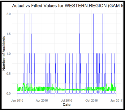
Figure 19: GAM Model
(Source: R Studio)

The graph illustrates the actual accident numbers (blue lines) in comparison to the fitted values using the GAM model (green line) for the WESTERN area. In contrast to the linear model, the GAM model accounts for local changes in accident patterns, demonstrating a superior match. Nonetheless, the increases in actual incidents remain inadequately reflected, indicating persistent patterns and possible underfitting. This suggests that the adaptable GAM is unable to properly encapsulate the non-linearities inherent in accident data, underscoring the necessity for more sophisticated models, including interaction terms or seasonal components.

Q.7.4 Comparison of the models

Figure 20: Comparison
(Source: R Studio)

AIC data show that the GAM model (AIC = 19103.07) matches better than the linear model (AIC = 19362.41). Non-linear patterns are better captured by the GAM model than the linear approach. GAM is better for accident analysis forecasts because meteorological variables and accident incidences are interconnected.

Q.7.5 Residual analysis

The GAM model residuals show patterns, indicating correlation. Clusters or patterns in residuals suggest model neglect of variability. Model efficacy may decrease due to time dependencies or omitted factors. This highlights the need for more advanced methods, such as time-series elements, to accurately depict accident dynamics and improve predictive precision.

Q7.6 Improvisation of predictor EHF

EHF quantifies the impact of severe heat on accident frequency, enhancing model fit and precision.

Q.7.7 Evaluation of EHF

EHF serves as a reliable predictor, as excessive heat can influence driver behaviour and vehicle performance, resulting in accidents. Nevertheless, supplementary meteorological variables such as precipitation, wind velocity, and visibility may possess greater forecasting capability. For example, precipitation can enhance road slipperiness, yet reduced sight can hinder driver reaction time. Incorporating precipitation into the model in conjunction with EHF allows us to evaluate whether it enhances model performance. An increase in model fit is suggested by a decrease in AIC with the inclusion of precipitation. This modification facilitates the capturing of a broader spectrum of meteorological factors impacting road safety, hence rendering the model more comprehensive for accident prediction.

Q.8 Reflection

Q.8.1 Recommendation of data

Additional data, including traffic density, road conditions, vehicle classifications, driver demographics, and accident severity, could substantially improve the model. Incorporating these characteristics would enhance the comprehension of accident causation, hence augmenting predictive efficacy and precision.

Q.8.2 Justification of the fulfilment of the research objectives

Indeed, my investigations have partially fulfilled the purpose by identifying critical meteorological variables influencing road accidents. Nevertheless, the models exhibit certain limits, suggesting that the inclusion of supplementary parameters could enhance prediction accuracy and reliability.

Q.8.3 Missing Value

In the presence of missing values, I would employ techniques such as mean or median imputed to provide continuous variables, mode imputation for categorical variables, or more sophisticated algorithms like KNN imputation and multiple imputation to maintain data integrity (Lee a& Yun, 2024).

Q.8.4 Overfitting

To address overfitting, I would employ approaches such as stepwise selection, regularisation methods (LASSO or Ridge regression), and cross-validation to minimise the number of explanatory variables, preserving just the most important predictors to enhance model generalisability (Laufer et al. 2023).  

References

STT500 Statistics for decision making Assignment 2 Sample

Description

The individual assignment must provide a 1500-word written report. This report for The Assignment Helpline will develop students' quantitative writing skills and test their ability to apply theoretical concepts covered from weeks 1-8. Please use Excel for statistical analysis in this assignment. Relevant Excel statistical output must be properly analysed and interpreted.

Assignment Data

The real estate markets present a fascinating opportunity for data analysts to analyse and predict property prices. Considering the data provided a large set of property sales records.

Attribute information:

PN: Property identification number • Price: Price of the property ($000) • Bedrooms: Number of bedrooms

• Bathrooms: Number of bathrooms

Lot size: Land size (in square meters)

The population property data from which you will select your sample data consists of 500 IDs each with an identifying property number (PN) ranging from 1 (or 001) to 500.

Your first task is to select 50 three-digit random (property) numbers ranging from 001 to 500 from the provided table of random numbers.

To select your 50 random property identification numbers, you will need to first go to a starting position row and column in the random number table. Defined by the last three digits of your Polytechnic Institute Australia student identification number. The last two digits of your PIA ID number identify the row, and the third last digit identifies the column of your (relatively) "unique" starting position.

You need to record these first three acceptable ID numbers into the first column of an Excel spreadsheet and then continue this process until fifty valid three-digit personal identification numbers are selected.

To select your sample data based on 50 randomly selected properties from the random number table, you will need to use these identification numbers to select properties from the Excel sheet of the population property data.

For the demonstration last three digits of 205, reading across row 05 from left to right starting at column 2 as instructed, you would encounter the following three-digit numbers.

04773 12032 51414 82384 38370 00249 80709 72605 67497

You need to record these first three acceptable ID numbers, 047, 120, 383 and 002 into the first column of an Excel spread-sheet and then continue this process until fifty valid three-digit personal identification numbers selected.

Students are required to use the generated data according to their student ID to answer the assessment questions.

Make sure the following questions are covered in the data analysis:

1) Create 50 randomly selected properties from the random number table based on your PIA ID number, you will need to use these identification numbers to select properties from the Excel sheet of the population property data. Use your data to answer questions 2-10.

2) Use Excel to create frequency distributions, Bar charts, and Pie charts for the number of bedrooms and bathrooms. Comment on the key findings.

3) What type of variable (Continuous, Discrete, Ordinal, or Nominal) is the number of bedrooms, and justify your answer.

4) Use Excel to create Histogram for the Price of the property and Land size (square ft lot). Also. Comment on the key findings.

5) Show descriptive summary statistics for the Price of the property in thousand dollars and Land size (square ft lot). Comment on the shape, canter, and spread of these two distributions.

6) Check the normality of the Price of the property data with three pieces of evidence.

7) Construct a 95% confidence interval for the population's average Price of the property, also Interpret the confidence interval.

8) Construct a 95% confidence interval for the population's average Land size (square ft lot) of the property, also Interpret the confidence interval.

9) Test whether the population's average Price of the property in thousand dollars is different from $530. Formulate the null and alternative hypotheses. State your statistical decision using the significant value (a) of 5%.

10) State your conclusion in context.

Solution

Task 1: Selecting Random Sample

1. Based on ID 20241288, last 3 digits are: 288, In my ID 88 identifies row and 2 identifies the
column in the random number table.

Data Table

Task 2: Use Excel to create frequency distributions

2. Frequency Distribution, Bar charts and Pie chart for number of Bedrooms and bathrooms

Task 2: Use Excel to Create Frequency Distributions

2. Frequency Distribution, Bar charts and Pie chart for number of Bedrooms and bathrooms

Table 1: Frequency Distribution
(Source: Ms Excel)

The key finding from the frequency distribution of bathrooms, therefore, is that number of bathrooms is an ordinal discrete variable, by which we mean that it is a ranked variable with defined, separate values (i. e. 1, 1. 5, 2 and so on). The bar chart shows the frequency and distribution of the number of bathrooms which is protracted to show the most frequently occurring bathroom count among the buildings. This aspect of the visualization is informative about how the bathroom availability is usually distributed in the properties and a way of giving an estimate of which bathroom count is more popular among the properties in the data set in helping to decipher the general pattern of these homes.

Figure 1: Bar chart of bedroom frequency Distribution
(Source: MS- EXCEL)

Interpretation: This bar chart relates to the distribution of the number of bedrooms in the properties. This bar advertises how many of them have a certain number of bedrooms. For instance if out of 100 properties the majority of them have 3 rooms, then the bar corresponding to 3 rooms shall be the highest. In particular, this visualization makes it easier to determine which frequency of bedrooms is typical of the sampled properties.

Figure 2: Barchart of Bathroom frequency Distribution
(Source: MS- EXCEL)

Key Findings: The key finding here is that the number of bathrooms is classified as an ordinal discrete variable because it represents a ranked order (from 1 to 4), and the values are discrete—indicating distinct, separate units without intermediate continuous values. Just as the frequency distribution of the bedroom, this bar chart shows the frequency distribution of the number of bathrooms in the properties. It will also show the range of the numbers of bathrooms most common among the households. This can be useful for comprehension of how the probability of access is divided with concern to the units in the data set.

3. Variable

The number of bathrooms is considered an ordinal discrete variable. This categorization is justified because the variable reflects a ranked order, where each value represents a meaningful progression or quantity of bathrooms. The numbers indicate a clear sequence, from fewer bathrooms to more, which inherently implies an order (ordinal). The values are discrete because they represent distinct, separate units—there are no fractional or continuous numbers between these specified values in this context. While 1.5 or 2.75 bathrooms are possible, the intervals between the listed values are specific and not continuous, further reinforcing the discrete nature of the variable.

4. Histogram of price of Property and land size

Key Findings :This histogram above illustrates the property prices and land sizes. By this, you are able to get a view of how these variables are distributed in that the height of the bars depict the number of properties in the given price or land size category. The shape of the histogram can also reveal whether the data is skewed, normally distributed and whether the data has some other special distribution. Here, the histogram effectively illustrates the distribution and dispersion of the data about property prices and land areas in order to detect the properties such as skewness, peak or any gaps.

5. Descriptive Summary Statistics

Table 2: Descriptive Summary Statistics of price of property
(Source : MS - Excel)

key Findings: The following table provides some of the property price summary measurements which include ‘mean’, ‘median’, ‘standard deviation’ and ‘range’. These measures provide essentials like the central tendencies and variability and also overall appearance of the distribution of property prices in the dataset. Average property price can be calculated using mean and median of the property prices and variability of the prices can be understood through, standard deviation. The range gives the variation of prices from the highest to the lowest, which shows the variation of the values.

Table 3: Descriptive Summary Statistics of Land Size
(Source : MS - Excel)

key Findings : In the same way as with price statistics, the following table gives an overview of some basic descriptive statistics of land size. They include such indicators as the arithmetic average, the median, and the standard deviation because they give a general idea of the size of the land within the established sample. The summary statistics of land size also assist in identifying the degree of dispersion of the land size proportional to properties being analyzed through the mean of the land size and the standard deviation.

6. Normality of the Price of Property Data with Three Pieces of Evidences

Figure 4 : Normality of the price of property Data with three pieces of evidences

(Source : MS EXCEL )

Key Findings:

This, most probably, represents a normality test – Q-Q plot, histogram, or a result of the Shapiro-Wilk test. The purpose is therefore to check the assumption that the property price data can be from a normal distribution. There will be three statistical measures to support or reject normality including histogram of the distribution, measuring the agreement of Q-Q plot and the p-value from a normality test. The condition is that data is normally distributed; it implies that a majority of house prices are exceptionally close to the average while very few prices are on the high or low end. If the data does not look like a normal distribution then further data transformation might be required or analyze the data using other statistical techniques.

7.

Interpretation :

This table gives the confidence interval of the average price of property. The confidence level is usually specified as 95% which means that the true population mean will, in all probability, lie within this range 95% of the time. This interval is important in determining the precision of the sample mean of the population mean. By using confidence intervals to generate hypotheses, it assists in estimating the population mean thus providing a range within which the mean property price lies.

8.

Table 5 : 95 % confidence interval for the population’s average Land Size
(Source : MS - Excel)

As is the case with the property price, this table shows the confidence interval for the average size of the land. It means the mean of the estimated average land size for the population has to be between that range with 95 percent confidence. A small interval provides more accuracy of the estimate as compared with the wide interval.

9.

Table 6: testing of population average price of property
(Source : MS - Excel)

Statistical Decision:

Interpretation: The following table will have the information of whether the null hypothesis should be rejected or not at a significance level (alpha) of 5% using the test statistic and p value. Most often, the p value is determined alongside the lower bound and if the p value gets less than 0. 05, the null hypothesis is being turned down which makes it clear that the average price of the property is significantly different from the set value.

10. Conclusion

This analysis gave a detailed description of property characteristics such as the distribution of the number of bedrooms and bathrooms, the price of the property and land area. These distributions described how frequent a particular combination of bedrooms and bathrooms were and in the analysis, bathrooms was determined to be an ordinal discrete variable because of the ranked and distinct values. Histograms of property prices and size of the land, represented the spread of the corresponding variable and can give an indication of the skewness of the variables. Descriptive statistics yielded measures of central tendency and variability which are important in the assessment of the overall frequency distribution of property prices and sizes of land. The results of the normality tests on property prices indicated that, even though data seemed more or less normally distributed, it was still necessary to conduct additional tests or transformations. The 95% confidence intervals were also employed to estimate the population means of property prices as well as land sizes to show the preciseness of the samples that were taken. Finally, hypothesis testing was used to ascertain whether the mean property price deviated by a statistically significant margin from a given value, in the overall population. Collectively, these analyses provide properties characteristics’ important information and provide practical references for real estate related industries.
 

STATS7061 Statistical Analysis Assignment Sample

Prepare short written responses to the following questions. Please note that you must provide a clear interpretation and explanation of the results for assignment help reported in your output.

Question 1 – Binomial Distribution

A university has found that 2.5% of its students withdraw without completing the introductory business analytics course. Assume that 100 students are registered for the course.

a) What is the probability that two or fewer students will withdraw?
b) What is the probability that exactly five students will withdraw?
c) What is the probability that more than three students will withdraw?
d) What is the expected number of withdrawals from this course?

Question 1

Here, number of trials (n) = 100
Probability of success i.e. student withdrawing from course (p) = 0.025
The various probabilities have been computed using BINOMIST function in Excel.

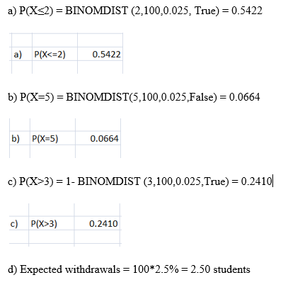
a) P(X≤2) = BINOMDIST(2,100,0.025,True) = 0.5422

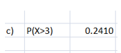
b) P(X=5) = BINOMDIST(5,100,0.025,False) = 0.0664

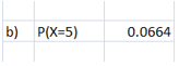
c) P(X>3) = 1- BINOMDIST(3,100,0.025,True) = 0.2410

d) Expected withdrawals = 100*2.5% = 2.50 students

Question 2 – Normal Distribution

Suppose that the return for a particular investment is normally distributed with a population mean of 10.1% and a population standard deviation of 5.4%.

a) What is the probability that the investment has a return of at least 20%?

b) What is the probability that the investment has a return of 10% or less?
A person must score in the upper 5% of the population on an IQ test to qualify for a particular
occupation.

c) If IQ scores are normally distributed with a mean of 100 and a standard deviation of 15, what score must a person have to qualify for this occupation?

Question 2

a) Mean = 10.1%
Standard deviation = 5.4%
The relevant output from Excel is shown below.

The z score is computed using the inputs provided. Using the NORMS.DIST(1.833) function, the probability of P(X<20%) has been determined. Finally, the probability that the return would be atleast 20% is 0.0334.

b) Mean = 10.1%
Standard deviation = 5.4%
The relevant output from Excel is shown below.

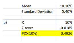
The z score is computed using the inputs provided. Using the NORMS.DIST(-0.0185) function, the probability of P(X<10%) has been determined. It can be concluded that there is a probability of 0.4926 that the given investment has a return of 10% or less.

c) The relevant output from Excel is shown below.

The requisite percentile score required is 95%. The corresponding Z value for this as determined using NORMS.INV has come out as 1.644854. This along with the mean and standard deviation has been used to derive the minimum qualification score as 124.67. Hence, to be in the top 5%, a candidate needs to score atleast 124.67 in the IQ test.

Question 3 – Normal Distribution

According to a recent study, the average night’s sleep is 8 hours. Assume that the standard deviation is 1.1 hours and that the probability distribution is normal.

a) What is the probability that a randomly selected person sleeps for more than 8 hours?
b) Doctors suggest getting between 7 and 9 hours of sleep each night. What percentage of the population gets this much sleep?

Question 3

a) The relevant output from Excel is shown below.

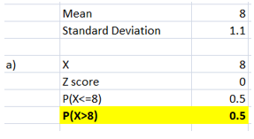
Using the mean, standard deviation and the X value, the Z score has been computed as zero. Using NORMS.DIST(0) function, the probability of P(X<=8) has come out as 0.5. Further, the probability of P(X>8) has been computed as 0.5. Hence, the probability that a randomly selected person sleeps more than 8 hours is 0.5.

b) The relevant output from Excel is shown below.

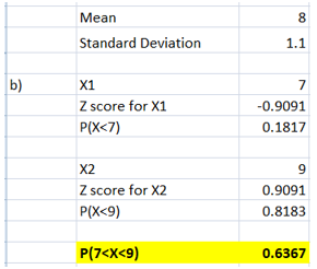
For X1 = 7 hours, the corresponding z score was computed followed by finding the P(X<7) using NORMS.DIST(-0.9091) function. For X2 = 9 hours, the corresponding z score was computed followed by finding the P(X<9) using NORMS.DIST(0.9091) function. The probability that people would be getting sleep between 7 and 9 hours is 0.6367. Thus, 63.67% of the population is getting sleep between the 7 and 9 hours each night.

Question 4 – Normal Distribution

The time needed to complete a final examination in a particular college course is normally distributed with a mean of 160 minutes and a standard deviation of 25 minutes. Answer the following questions:

a) What is the probability of completing the exam in 120 minutes or less?

b) What is the probability that a student will complete the exam in more than 120 minutes but less than 150 minutes?

c) What is the probability that a student will complete the exam in more than 100 minutes but less than 170 minutes?

d) Assume that the class has 120 students and that the examination period is 180 minutes in length. How many students do you expect will not complete the examination in the allotted time?

Question 4

a) The relevant output from Excel is shown below.

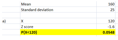
For X =120, the corresponding z score was computed followed by finding the P(X<=120) using NORMS.DIST(-1.6) function. The probability of completing the exam in 120 minutes or lesser is 0.0548.

b) The relevant output from Excel is shown below.

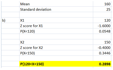
For X1 = 120 minutes, the corresponding z score was computed followed by finding the P(X<120) using NORMS.DIST(-1.6) function. For X2 = 150 minutes, the corresponding z score was computed followed by finding the P(X< 150) using NORMS.DIST(-0.40) function. The probability that a student will complete the test in more than 120 minutes but less than 150 minutes is 0.2898.

c) The relevant output from Excel is shown below.

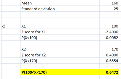
For X1 = 100 minutes, the corresponding z score was computed followed by finding the P(X<100) using NORMS.DIST(-2.4) function. For X2 = 170 minutes, the corresponding z score was computed followed by finding the P(X< 170) using NORMS.DIST(0.40) function. The probability that a student will complete the test in more than 100 minutes but less than 170 minutes is 0.6472.

d) The relevant output from Excel is shown below.

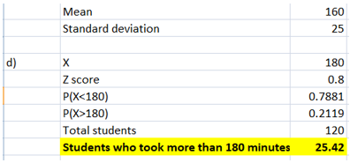
For the score of 180 minutes, the corresponding Z score is 0.8. Using NORMS.DIST(0.8), the P(X<180) is 0.7881. Hence, the probability of student taking more than 180 minutes or not finishing within the allotted 180 minutes is 0.2119. The total number of students given is 120. Thus, students not finishing within the allotted 180 minutes is 0.2119*120 = 25.42 or 26 students.

Statistical Analysis Assignment Sample

INSTRUCTIONS

Perform the required calculations using Excel (and PHStat where appropriate), present your findings (i.e., the relevant output), and prepare short written responses to the following questions. Please note that you must provide a clear interpretation and explanation of the results reported in your output. Please submit your answers in a single Word file.

Question 1 – Binomial Distribution (8 marks)

A university has found that 2.5% of its students withdraw without completing the introductory business analytics course. Assume that 100 students are registered for the course.

a) What is the probability that two or fewer students will withdraw?
b) What is the probability that exactly five students will withdraw?
c) What is the probability that more than three students will withdraw?
d) What is the expected number of withdrawals from this course?

Question 2 – Normal Distribution

Suppose that the return for a particular investment is normally distributed with a population mean of 10.1% and a population standard deviation of 5.4%.
a) What is the probability that the investment has a return of at least 20%?
b) What is the probability that the investment has a return of 10% or less?
A person must score in the upper 5% of the population on an IQ test to qualify for a particular occupation.
c) If IQ scores are normally distributed with a mean of 100 and a standard deviation of 15, what score must a person have to qualify for this occupation

Question 3 – Normal Distribution (4 marks)

According to a recent study, the average night’s sleep is 8 hours. Assume that the standard deviation is 1.1 hours and that the probability distribution is normal.
a) What is the probability that a randomly selected person sleeps for more than 8 hours?
b) Doctors suggest getting between 7 and 9 hours of sleep each night. What percentage of the population gets this much sleep?

Question 4 – Normal Distribution (10 marks)

The time needed to complete a final examination in a particular college course is normally distributed with a mean of 160 minutes and a standard deviation of 25 minutes. Answer the following questions:

a) What is the probability of completing the exam in 120 minutes or less?
b) What is the probability that a student will complete the exam in more than 120 minutes but less than 150 minutes?
c) What is the probability that a student will complete the exam in more than 100 minutes but less than 170 minutes?
d) Assume that the class has 120 students and that the examination period is 180 minutes in length. How many students do you expect will not complete the examination in the allotted time?

Solution

Question 1

Here, number of trials (n) = 100
Probability of success i.e. student withdrawing from course (p) = 0.025
The various probabilities have been computed using BINOMIST function in Excel.

Question 2

a) Mean = 10.1%
Standard deviation = 5.4%
The relevant output from Excel is shown below.

The z score is computed using the inputs provided. Using the NORMS.DIST(1.833) function, the probability of P(X<20%) has been determined. Finally, the probability that the return would be atleast 20% is 0.0334.

b) Mean = 10.1%
Standard deviation = 5.4%
The relevant output from Excel is shown below for assignment help

The z score is computed using the inputs provided. Using the NORMS.DIST(-0.0185) function, the probability of P(X<10%) has been determined. It can be concluded that there is a probability of 0.4926 that the given investment has a return of 10% or less.

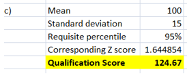
c) The relevant output from Excel is shown below.

The requisite percentile score required is 95%. The corresponding Z value for this as determined using NORMS.INV has come out as 1.644854. This along with the mean and standard deviation has been used to derive the minimum qualification score as 124.67. Hence, to be in the top 5%, a candidate needs to score atleast 124.67 in the IQ test.

Question 3

a) The relevant output from Excel is shown below.

Using the mean, standard deviation and the X value, the Z score has been computed as zero. Using NORMS.DIST(0) function, the probability of P(X<=8) has come out as 0.5. Further, the probability of P(X>8) has been computed as 0.5. Hence, the probability that a randomly selected person sleeps more than 8 hours is 0.5.

b) The relevant output from Excel is shown below.

For X1 = 7 hours, the corresponding z score was computed followed by finding the P(X<7) using NORMS.DIST(-0.9091) function. For X2 = 9 hours, the corresponding z score was computed followed by finding the P(X<9) using NORMS.DIST(0.9091) function. The probability that people would be getting sleep between 7 and 9 hours is 0.6367. Thus, 63.67% of the population is getting sleep between the 7 and 9 hours each night.

Question 4

a) The relevant output from Excel is shown below.

For X =120, the corresponding z score was computed followed by finding the P(X<=120) using NORMS.DIST(-1.6) function. The probability of completing the exam in 120 minutes or lesser is 0.0548.

b) The relevant output from Excel is shown below.

For X1 = 120 minutes, the corresponding z score was computed followed by finding the P(X<120) using NORMS.DIST(-1.6) function. For X2 = 150 minutes, the corresponding z score was computed followed by finding the P(X< 150) using NORMS.DIST(-0.40) function. The probability that a student will complete the test in more than 120 minutes but less than 150 minutes is 0.2898.

c) The relevant output from Excel is shown below.

For X1 = 100 minutes, the corresponding z score was computed followed by finding the P(X<100) using NORMS.DIST(-2.4) function. For X2 = 170 minutes, the corresponding z score was computed followed by finding the P(X< 170) using NORMS.DIST(0.40) function. The probability that a student will complete the test in more than 100 minutes but less than 170 minutes is 0.6472.

d) The relevant output from Excel is shown below.

For the score of 180 minutes, the corresponding Z score is 0.8. Using NORMS.DIST(0.8), the P(X<180) is 0.7881. Hence, the probability of student taking more than 180 minutes or not finishing within the allotted 180 minutes is 0.2119. The total number of students given is 120. Thus, students not finishing within the allotted 180 minutes is 0.2119*120 = 25.42 or 26 students.

BEO1106 Business Statistics Assignment Sample

Introduction

The price of a property can be determined by a number of factors (in addition to the market
trend). These factors may include (but not the least): The location, the land size, the size of the built area, the building type, the property type, number of rooms, number of bathroom and toilets, swimming pool, tennis court and so on.

The sample data you collected for your assignment contain the following variables:

V1 = Region where property is located (1 = North, 2 = West, 3 = East, 4 = Central)
V2 = Property type (0 = Unit, 1 = House)
V3 = Sale result (1 = Sold at auction, 2 = Passed-in, 3 = Private sale, 4 = Sold before auction).
Note that a blank cell for this variable indicates that the property did not sell.
V4 = Building type (1 = Brick, 2 = Brick veneer, 3 = Weatherboard, 4 = Vacant land)
V5 = Number of rooms
V6 = Land size (Square meters)
V7 = Sold Price ($000s)
V8 = Advertised Price ($000s).

Requirement

In relation to the Simple Regression topic of Business Statistics, for this Case Study, you are
required to conduct a regression analysis to estimate the relation between Number of Rooms and Advertised Price of properties in Melbourne.

Instruction

You need to prepare a sample data using the Number of Rooms and the Advertised Price variables. You may find that V5 (Number of Rooms) variable has some missing observations in your sample. In order for Excel to estimate a regression equation, Excel requires a balanced data set. This means that both dependent variables and independent variables must have the same (balanced) number of observations in the data set. To balance the data set, we have to remove the observations which contain missing data. Refer to the steps in the Excel file Regression Estimation example for Case Study.xlsx to assist you to construct your balanced sample data set for the regression analysis.

Task 1

In the Answer Sheet provided, name the dependent variable (Y) and the independent variable (X). Provide a brief explanation for assignment help to support your choice.

Task 2

In a sentence, explain whether you expect a positive or a negative relation between the X and the Y variables.

Task 3

Use Excel to produce a scatterplot using the independent variable for the horizontal (X) axis and the dependent variable as the vertical (Y) axis. Copy and paste the scatterplot to the Answer Booklet.

Hint: Follow the graph presentation (in Step 5, Regression Estimation example for Case
Study.xlsx).

Note:Title of the scatterplot and the labels for axes will account for 0.5 mark for each.

Task 4

Follow the Excel procedure (select Data / Data Analysis / Regression) outlined on seminar note Slide 16, using the X variable and the Y variable you nominated in Task 1, generate regression estimation output tables. Copy the Regression Statistics and Coefficients tables (refer to Slide 27 and Slide 28) to the Answer Booklet.

Task 5

Refer to the Regression Statistics table in Task 4, briefly describe the strength of the correlation between X and Y variables. Ensure your statement is supported by the statistic figure from the table.

Task 6

Does the information shown in the Coefficients table agree with your expectation in Task 2?
Briefly explain the reasoning behind your answer.

Task 7

Refer to the Coefficients table, and follow the presentation on seminar note Slide 19, construct the least squares linear regression equation for the relationship between the independent variable and the dependent variable.

Task 8

Interpret the estimated intercept and the slope coefficients.

Task 9

Select one of the two following scenarios which describe your choice in Task 1.

• In Task 1, if you nominated Number of Rooms is the independent variable, then you are asked to estimate the Advertised Price (dependent variable) of a property given the number of rooms of the property is 5.

• In Task 1, if you nominated Advertised Price is the independent variable, then you are asked to estimate the Number of Rooms (dependent variable) of a property given the advertised price is $1.55 (million).

Task 10

With reference to the R Square value provided in the Regression Statistics table, explain whether you would trust your estimation in Task 9. Comment on whether your answer in Task10 agrees with the answer in Task 5 in terms of the strength of the linear relationship between X and Y.

Task 11

State, symbolically, the null and alternative hypotheses for testing whether there is a positive linear relationship between Number of Rooms and Advertised Price in the population.

Task 12

Use the Empirical Rule, state the z- value which is corresponding to 2.5% significant level.

Task 13

Use the p-value approach to decide, at a 2.5% level of significance, whether the null hypothesis of the test referred to in Task 11 can be rejected (or not). Make sure you provide a justification for your decision.

Task 14

Following the decision in Task13, provide a precise conclusion to the hypothesis test conducted in Task 13.

Task 15

From information provided in the Coefficients table, construct a 95% confidence interval estimate of the gradient of the population regression line. Is this interval consistent with the conclusion to the hypothesis test you arrived at in Task 14? Briefly explain the reasoning behind your answer

Solution

STA201 Business Statistics Assignment Sample

Assessment - Analytics Assignment

Individual/Group - Individual
Length - 1000 Words

Learning Outcomes - The Subject Learning Outcomes demonstrated by successful completion of the task below include:

a) Produce, analyse, and present data graphically and numerically, and perform statistical analysis of central tendency and variability.

b) Apply inferential statistics to draw conclusions about populations, including confidence levels, hypothesis testing, analysing variance and comparing with benchmarks in decision making processes.

c) Measure uncertainty, including continuous and discrete probability and sampling distributions to select appropriate methods of data analysis.

d) Apply parametric tests and analysis techniques to determine causation and forecasting to assist decision making.

e) Utilise technology to analyse and manipulate data and present findings to peers and other stakeholders.
Submission Due by 11:55 pm AEST/AEDT Sunday end of Module 6.2 (Week 12).

Weighting - 30%

Assessment Tasks for assignment help

1. Prepare a summary statistics table and discuss the central tendency and variations for all variables.

2. Plot the dependent variable (house price), against each independent variable using scatter plot/dot function in Excel. Comment on the strength and the nature of the relationship between the dependent and the independent variables.

3. Generate a multiple regression summary output. Using the information on regression output, state the multiple regression equation.

4. Interpret the meaning of slope coefficients of independent variables.

5. Interpret the R 2 and adjusted R 2 of your model.

6. Conduct a test for significance of your overall multiple regression model at the 0.05 level of significance. You must state your null and alternative hypotheses.

7. At the 0.05 level of significance, determine whether each independent variable makes a significant contribution to the regression model. Based on these results, indicate the independent variables to include in this model.

8. Construct a 95% confidence interval estimate of population slope of house prices withproperty size. Interpret your results.

9. Construct a 95% confidence interval estimate of population slope of house prices with distance to nearest train station. Interpret your results.

10. Choose one of the houses currently advertised for sale in your chosen suburb (the one to collect the data of). Make sure to choose a house whose asking price is also advertised. Predict the price of the house using the regression equation you generated in part 3 and values of the independent variables as advertised. Compare the predicted price with the asking price.

Solution

Task 1: summary statistics:

As per the table 1 in appendix, it can be seen that mean value of sale price is $465542 with median $422500 and mode $420000. Hence, the average sales price is $465542, whereas most of the property price is $420000, thus the data is not normally distributed. Standard deviation is 141997.29 and sample variance is 20163229016.33. Thus, the housing sales price has very high variability in it. Kurtosis value of 3.09 signifies the fact that there are outliers and range of $790000 also demonstrates maximum and minimum housing price has very high difference in it (Bono et al., 2019). Mean value of bedroom is 3.78 with mode 4.

Average bedroom number is 3.78 whereas most of the property has 4 bedrooms. Standard deviation and sample variance is 0.51 and .26 respectively. Thus, the variation in data of bedroom is low. Kurtosis value is 2.42 that showcase there is low number of outliers with negative skewness that has right tail. Bathroom average count is 1.86 with mode 2. Thus, most of the houses has 2 bathrooms with average value of bathroom 1.86. Low standard deviation of 0.45 and sample variance of 0.20 showcase bathroom data has limited variability. Kurtosis value is 1.39 with range of 2 showcase there is low to moderate variability in the bathroom count data.

Property size has mean value of 791.40 m2 with mode752 m2 and median of 751 m2. Thus, most of the property size is 751 m2 with average value of 791.40 m2. Standard deviation and sample variance is very high that showcase property size has high variability. Kurtosis value of 34.49 and range of 3837 showcase there is very high variability in property size data. As per skewness of 5.37, data is highly skewed, and it has left tail. Average distance of property from metro station is .46 km, however, as per mode, most of the property has average distance of .43 km. Thus, the data is normally distributed, and it has low variability with standard deviation of .29 and sample variance of .08. Kurtosis of 4.05 demonstrates there is outliers and range signifies that the data has low variability in it.

Task 2: plotting dependent variables against independent variable:

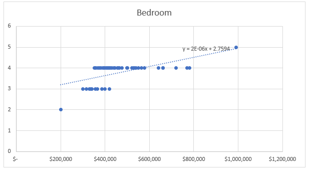
Figure 1: Association between number bedroom and property price

Figure 1 demonstrates the association between bedroom and property price. Though the plots did not showcase anything clearly, however, an upward sloping trend line demonstrated a positive association between the variables (Schober et al., 2018). Positive association demonstrates increase in number of bedrooms, increase the housing price.

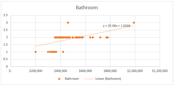
Figure 2: Association between bathroom number and property price

As per the figure 2 it can be seen that there is also an upward trend in price as the number of bathroom increases. Hence, the association is positive, however the degree of association is not clear from here.

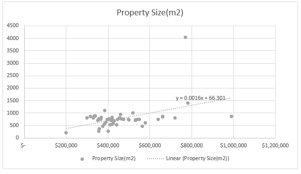
Figure 3: Association between property size and property price

Figure 3 demonstrated as the property size increase; price of property also increase. However, the plots are not scattered demonstrating, as the property size increase price of property does not increase moderately. Hence, though the trend line showcase a positive association between two values, yet the degree of association is not very high.

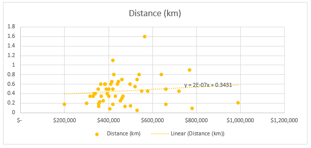
Figure 4: Association between distance from metro and property price

Figure 4 demonstrates a positive association between the distance from metro and property price. Hence, with rise in distance of property from metro, price tends to rise. However, as the distance increase, housing price does not increase proportionately as per plot demonstrating a weak association.

Task 3: Multiple regression:

To develop model that can predict the housing price based on independent variables, multiple regression has been done here. As per table 2 in appendix, following regression model can be mentioned:

Y = -169462.44 + 104230.45 * X1 + 80772.80 * X2 + 100.18 * X3 + 25196.60 * X4 [Where, Y is property price, X1 is bedroom number, X2 is bathroom number, X3 is property size and X4 is distance from metro]

Task 4: Slope coefficient interpretation:

As per table 2, slope coefficient of bedroom is 104230.45 which mean, change in 1 unit of bedroom can lead the property price to increase by $104230.45. Slope coefficient of bathroom demonstrates 1 unit of bathroom addition can lead to rise in house price by $80772.80. As per property size slope coefficient, 1 m2 rise in property size increase the property price by $100.18. Distance slope coefficient, 1 km rise in distance can increase the housing price by $25196.60.

Task 5: R2 and adjusted R2 model:

R square value of the model is 0.53, which mean independent variables can explain 53% of variability of the data in dependent variable. Adjusted R Square demonstrates how additional independent variable can change the predictability of the model for dependent variable (Sharma et al., 2021). Adjusted R Square value of 0.49, means addition of exploratory variables can actually fails to make the model more significant in predicting variability of data.

Task 6: Test of significance of model:

Null hypothesis: H0: Fit of intercept only model is equal to predicted model

Alternative hypothesis: H1: Fit of intercept only model is significantly reduced compared to predicted model
As per the ANOVA in table, F value is 0.00, which is lower than critical value of 0.05. Hence, the model is a good fit model and null hypothesis is accepted here.

Task 7: Test of significance of independent variable:

At 0.05 level of significance, as per table 2, only bedroom and property size seems to significantly influence the property price as their p value is 0.02 and 0.00 respectively. For other exploratory variables, p value is 0.1 (for bathroom) and 0.62 (for distance) which is higher than critical value of 0.05. Thus, bathroom and distance cannot significantly influence the property price.

Considering the significance of bedroom and property size, these factors can only be included in the regression model; thus, the revised regression model is as follows:

Y = -169462.44 + 104230.45 * X1 + 100.18 * X3

Task 8: 95% confidence interval of property size:

Confidence interval = b1 ± t(1-α)/2, n-2 * se(b1)
At 95% confidence interval, t(1-α)/2, n-2 = 2.011
b1 = 100.18
se(b1) = 28.92
Confidence interval = 100.18 ± 2.011 * 28.92 = 58.13
Confidence interval = 100.18 ± 58.13 = 158.13, 42.05

So, with 95% confidence interval, one m2 change in property size change the housing price between $158.13 and $42.05.

Task 9: 95% Confidence interval of distance:

Confidence interval = b1 ± t(1-α)/2, n-2 * se(b1)
At 95% confidence interval, t(1-α)/2, n-2 = 2.011
b1 = 25196.60
se(b1) = 51167.47

Confidence interval = 25196.60 ± 2.011 * 51167.47 = 128094.38, -77701.18

So, with 95% confidence interval it can be said that with 1 km change in distance, housing price change between $128094.38 and -$77701.18.

Task 10: Estimation of House Price:

House price at Clayton with 3-bedroom, 1 bathroom, 191 m2 property size and .5 km distance to metro:

Y = -169462.44 + 104230.45 * 3 + 100.18 * 191 = $162363.61

Hence, the estimated property price at Clayton would be $162363.31

Reference:

HI6007 Statistics for Business Decisions Assignment Sample

Assignment Specifications

Purpose:

This assignment aims at assessing students’ understanding of different qualitative and quantitative research methodologies and techniques. Other purposes are:

1. Explain how statistical techniques can solve business problems

2. Identify and evaluate valid statistical techniques in a given scenario to solve business problems

3. Explain and justify the results of a statistical analysis in the context of critical reasoning for a business problem solving

4. Apply statistical knowledge to summarize data graphically and statistically, either manually or via a computer package

5. Justify and interpret statistical/analytical scenarios that best fit business solution

Instructions:

• Your assignment must be submitted in WORD format only.

• When answering questions, wherever required, you should copy/cut and paste the Excel output (e.g., plots, regression output etc.) to show your working/output. Otherwise, you will not receive the allocated marks. Moreover, you must attach your excel file which includes data, output etc.

• You are required to keep an electronic copy of your submitted assignment to re-submit, in case the original submission is failed and/or you are asked to resubmit.

• Please check your Holmes email prior to reporting your assignment mark regularly for possible communications due to failure in your submission.

Group Assignment Questions for Assignment Help

Assume your group is the team of data analytics in a renowned Australian company. The company offers their assistance to distinct group of clients including (not limited to), public listed companies, small businesses, educational institutions etc. Company has undertaken several data analysis projects and all the projects are based on multiple regression analysis.
Based on the above assumption, you are required to.

1. Develop a research question which can be addressed through multiple regression analysis.

2. Note: This should be a novel research question and you are not allowed to directly copy from internet.

3. Explain the target population and the expected sample size

4. Briefly describe the most appropriate sampling method.

5. Create a data set (in excel) which satisfy the following conditions. (You are required to upload the data file separately).

a. Minimum no of independent variables – 2 variables

b. Minimum no of observations – 30 observations

Note: You are required to provide information on whether you used primary or secondary data,
data collection source etc.

3. Perform descriptive statistical analysis and prepare a table with following descriptive measures for all the variables in your data set. Mean, median, mode, variance, standard deviation, skewness, kurtosis, coefficient of variation.

4. Briefly comment on the descriptive statistics in the part (5) and explain the nature of the distribution of those variables. Use graphs where necessary.

5. Derive suitable graph to represent the relationship between dependent variable and each independent variable in your data set. (ex: relationship between Y and X1, Y and X2 etc)

6. Based on the data set, perform a regression analysis and correlation analysis, and answer the questions given below.

a. Derive the multiple regression equation.
b. Interpret the meaning of all the coefficients in the regression equation.
c. Interpret the calculated coefficient of determination.
d. At 5% significance level, test the overall model significance.
e. At 5% significance level, assess the significance of independent variables in the model.
f. Based on the correlation coefficients in the correlation output, assess the correlation
between explanatory variables and check the possibility of multicollinearity.

Solution

Introduction:

Under the changing business scenario, firms are now concerned about making strategies with the factors that actually influence their market value. Though there are various factors that can influence the market value, core factors like profit, sales and asset value are considered to be major element that has direct impact on market value. There has been considered able amount of research that demonstrates association between market value and various core factors; however, there is very limited study that demonstrate the relation for the Indian companies. Hence, to demonstrate the association between market value with the profit, sales and asset from the perspective of the Indian public listed companies, present study has been done. To perform the study, here statistical analysis has been done using excel where descriptive statistics and inferential statistical analysis has been used.

Research Question:

Research question of the present study is as follows:

How the market value of the Indian public listed companies is influenced by the profit, sales value and asset value of the company?

Target population and sample size:

In the present study Indian public listed companies enlisted in the Forbes 2000 list has been considered (Forbes.com 2021). As per the list, there were total 50 Indian companies who have successfully endured during the pandemic and performed best to be in top 2000 companies in the world (Forbes.com 2021). Thus, the population size of the study is 50 and considering 95% confidence interval with 5% margin of error, 45 observation has been considered as the sample for final study dataset.

Sampling method:

In the contemporary research work, sampling has various approach and they can be classified into two major groups, probability sampling and non-probability sampling. If the sample size considered based on randomisation, then it is probability sampling, whereas, if the sample size is decided by the convenience of the researcher, then it is non probability sampling (Etikan and Babtope 2019, p1006(2-5)). In case of probability sampling, it can further be divided into four types, which are random sampling, systematic sampling, stratified sampling and cluster sampling. For the present study, researcher has considered sample based on the randomisation, hence, the probability sampling has been considered and as the researcher has selected data randomly, from the population, thus it can be mentioned that sampling method has followed random sampling approach. Choosing non-probability sampling would make the bias selection of the data by the researcher making validity of the finding invalid. On the other hand, choosing systematic, stratified or clustered sampling is not justified as researcher has not made any group for the purpose of analysis. Thus, random sampling is the justified option for choosing sample.

Dataset creation:

Present study has considered data from the Forbes 2000 list where top 2000 public listed companies from world has been presented (Forbes.com 2021). As the dataset has been collected from the online source, thus secondary data collection approach has been used for making the dataset (Olabode et al. 2019, p(28(2)). The complete dataset available in Forbes provides country and industry wise top public listed company names who has exceled during pandemic. From this online data source, dataset from present study has been considered where four major variables were present which are:

• Market value
• Profit
• Sales value
• Asset value

All the values of the chosen variables have been presented in the form of Billion $. For making the dataset, first all available Indian public listed companies in the Forbes 2000 list have been considered and then through the random sampling, 45 companies have been used for making final sample dataset (Forbes.com 2021). For the further analysis, market value has been marked as the dependent variable, and profit, sales value and asset value has been marked as independent variable.

Descriptive statistical analysis:

Comment on descriptive statistics:

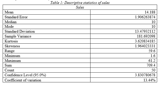
As per the descriptive statistics of sales it can be seen that mean value of annual sales of the Indian public listed companies is 14.18 billion $ with standard deviation 13.47 and variance 181.69; hence, the Indian public listed firms have high variability in sales value (Acosta et al. 2020, p3(3)). Median is 10 and mode is 10; hence most of the firms have profit of 10 billion $. As per the kurtosis and skewness, it can be seen that data has outlier and there is right tail. High range of 59.6 demonstrates, upper and lower sales value has high difference that satisfies the fact that sales data has high variability in it. Comparing the coefficient of variation, it can be stated that it has lower variation in data compared to other variables.

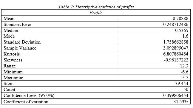
As per the descriptive statistics of profits it can be seen that mean value of annual profit of the Indian public listed companies is .79 billion $ with standard deviation 1.75 and variance 3.09; hence, the Indian public listed firms have low variability in profit value. Median is .54 and mode is 1.6; hence most of the firms have profit of .536 billion $. As per the kurtosis and skewness, it can be seen that data has outlier and there is left tail. Moderate range of 12.3 demonstrates, upper and lower profit value has low difference that satisfies the fact that profit data has low variability in it. Comparing the coefficient of variation, it can be stated that it has highest variation in data compared to other variables.

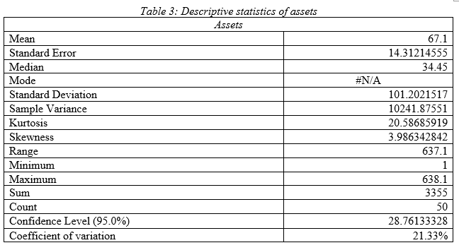
As per the descriptive statistics of assets value it can be seen that mean value of annual asset value of the Indian public listed companies is 67.1 billion $ with standard deviation 101.20 and variance 10241.87; hence, the Indian public listed firms have very high variability in assets value. Median is 34.45; hence most of the firms have asset value of 34.45 billion $. As per the kurtosis and skewness, it can be seen that data has outlier and there is right tail. High range of 637.1 demonstrates, upper and lower asset value has very high difference that satisfies the fact that asset value data has high variability in it. Comparing the coefficient of variation, it can be stated that it has high variation in data compared to other variables.

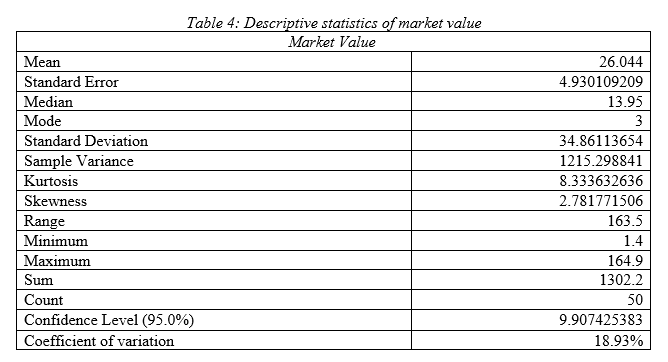
As per the descriptive statistics of market value it can be seen that mean value of annual market value of the Indian public listed companies is 26.04 billion $ with standard deviation 34.86 and variance 1215.29; hence, the Indian public listed firms have high variability in market value. Median is 13.95 and mode is 3; hence most of the firms have market value of 10 billion $. As per the kurtosis and skewness, it can be seen that data has outlier and there is right tail. High range of 163.5 demonstrates, upper and lower market value has high difference that satisfies the fact that market value data has high variability in it. Comparing the coefficient of variation, it can be stated that it has moderate variation in data compared to other variables.

Graphical presentation of association between dependent and independent variable:

In order to represent the association between the dependent variable (market value) and independent variable (profit, assets and sales value), graphical presentation has been used.

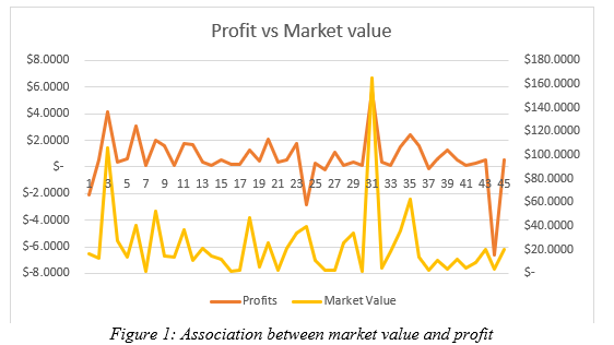
As per the figure 1, it can be seen that there is a good association between the market value and profit. As the profit of different firm changed, market value of the same has changed also. Major spikes can be seen for the 3rd, 31st and 43rd firm, where high change in the profit, and market value can be seen; however, the changes, is unidirectional. This means, overall change in the profit has resulted in change in market value in same direction.

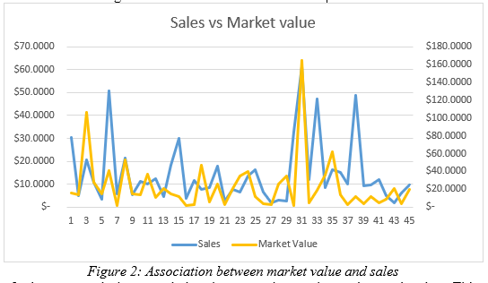
Figure 2 demonstrated the association between the market value and sales. This figure demonstrates a positive association between the dependent and independent variable. As the change occurred in sales value among the chosen Indian public listed companies, market value of the same has also changed. However, it is also important to mention that, there are some firms like 15th, 31st, 37th to 41st firm, where change in the sales value has not demonstrated identical change in market value. Thus, though the association between dependent and independent variable is positive, yet they are not very strong.

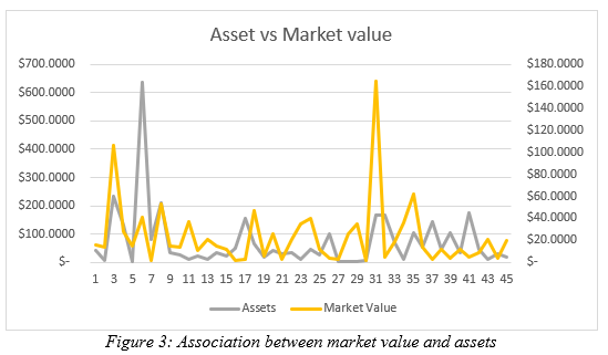
Figure 3 demonstrated association between the asset and market value. Here also change in asset price of the Indian public listed companies represent positive change in market value. However, it is also important to mention that there are certain companies like 5th, 31st, 21st to 25th, where change in asset price has been high, where as market value change has been very low. This demonstrates, though the association between asset price and market value is positive, yet it is not very strong.
Using the figure 3,

Regression analysis:

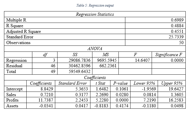
a.

As per the regression output presented in table 5, following regression equation can be formed:
Y = 8.84 + 0.72x1 + 11.74x2 – 0.03x3
[Y represents the dependent variable market value, x1 is sales value, x2 is profit value and x3 is asset value]

b.

As per the outcome of the table 5, intercept term has been found to be 8.84; this means, even if the sales, profit and asset is nil, market value will be 8.84 billion $ for the Indian public listed companies. Sales coefficient demonstrates that, with change in each billion $ of sales, market value will be increased by .72 billion $. Coefficient of profits of 11.74 demonstrates, change in each billion $ of profit will lead to rise in market value of the Indian public listed companies by 11.74 billion $. Lastly, coefficient of -0.03 for assets, determines that change in each billion $ of assets can lead to change in market value by .03 billion dollars negatively; hence, if there is rise in asset, there will be fall in market value and vis-à-vis (Chicco et al., 2021, p6(2-3)).

c.

As per the table 5 outcome, coefficient of determination, which is R Square has been found to be 0.49. This defines that, independent variable in regression model developed can explain 56% of variability in the data of dependent variable (Kadim et al., 2020, p860(2)).

d.

At 5% level, F value significance has been found to be 0.00 and the F value is 14.64. Thus, the model is significant and a good fit model.

e.

At 5% significance level, independent variable can be considered to be significant, if the p value is lower than 0.05, which is critical value. As per the output in table 5, p value of sales has been 0.02, p value of profits has been 0.00 and p value of assets has been 0.41 respectively (Miko 2021, p2(3)). Hence, at 5% level of significance, sales and profit can significantly influence the market value as their p value is lower than 0.05.

f.

To check the multicollinearity, Variance Inflation Factors (VIF) has been used (Shrestha 2020, p39(2)).
VIF = 1/(1 – R Square) = 1/(1-.48) = 1/.52 = 1.92
As per the calculated VIF, it is lower than 5, hence there is multicollinearity.

Conclusion:

As per the analysis, it has been found that there is positive association between the market value and independent variables like sales, profit and asset value. Though the association between dependent and independent variables are positive, yet, the association for market value with sales and asset is weak. As per the regression analysis, it can also be seen that assets do not influence the market value significantly, whereas, profit and sales can influence the market value significantly.

Reference:

A Kadim, N Sunardi, T Husain (2020), The modeling firm's value based on financial ratios, intellectual capital and dividend policy, Accounting, 6(5), pp.859-870. http://m.growingscience.com/ac/Vol6/ac_2020_48.pdf

B Miko (2021), Assessment of flatness error by regression analysis, Measurement, 171, p.1 - 10. https://www.sciencedirect.com/science/article/pii/S0263224120312264

Chicco, D., Warrens, M.J. and Jurman, G., 2021. The coefficient of determination R-squared is more informative than SMAPE, MAE, MAPE, MSE and RMSE in regression analysis evaluation. PeerJ Computer Science, 7, p.e623. https://peerj.com/articles/cs-623/

Forbes.com 2021. GLOBAL 2000, The World's Largest Public Companies. Available at: https://www.forbes.com/global2000/#3f01c42f335d

I Etikan, O Babtope (2019), A basic approach in sampling methodology and sample size calculation, Med Life Clin, 1(2), p.1006. http://www.medtextpublications.com/open-access/a-basic-approach-in-sampling-methodology-and-sample-size-calculation-249.pdf

MN Acosta Montalvo, MA Andrade, E Vazquez, F Sanchez, F Gonzalez-Longatt, JL Rueda Torres (2020), Descriptive Statistical Analysis of Frequency control-related variables of Nordic Power System. https://openarchive.usn.no/usn-xmlui/bitstream/handle/11250/2758995/2020GonzalezLongattDescriptive_POSTPRINT.pdf?sequence=4&isAllowed=y

N Shrestha (2020), Detecting multicollinearity in regression analysis, American Journal of Applied Mathematics and Statistics, 8(2), pp.39-42. https://www.researchgate.net/profile/Noora-

Shrestha/publication/342413955_Detecting_Multicollinearity_in_Regression_Analysis/links/5eff2033458515505087a949/Detecting-Multicollinearity-in
-Regression-Analysis.pdf

SO Olabode, OI Olateju, AA Bakare (2019), An assessment of the reliability of secondary data in management science research, International Journal of Business and Management Review, 7(3), pp.27-43. https://www.researchgate.net/profile/Akeem Bakare 2/publication/344346438_AN_ASSESSMENT_OF_THE_RELIABILITY_OF_SECONDARY_DATA_IN_MANAGEMENT
_SCIENCE_RESEARCH/links/5f6a7ff0a6fdcc0086346109/
AN-ASSESSMENT-OF-THE-RELIABILITY-OF-SECONDARY-DATA-IN-MANAGEMENT-SCIENCE-RESEARCH

STAT6000 Statistics for Public Health Assignment Help

Assignment Brief

Length 2000
Learning Outcomes:

This assessment addresses the following learning outcomes:

1. Understand key concepts in statistics and the way in which both descriptive and inferential statistics are used to measure, describe and predict health and illness and the effects of interventions.

2. Apply key terms and concepts of statistics for assignment help including; sampling, hypothesis testing, validity and reliability, statistical significance and effect size.

3. Interpret the results of commonly used statistical tests presented in published literature.

Submission Due Sunday following the end of Module 4 at 11:55pm AEST/AEDT*

Weighting - 30%
Total Marks - 100 marks

Instructions:

This assessment requires you to read two articles and answer a series of questions in no more than 2000 words. Most public health and wider health science journals report some form of statistics. The ability to understand and extract meaning from journal articles, and the ability to critically evaluate the statistics reported in research papers are fundamental skills in public health.

Read the Riordan, Flett, Hunter, Scarf and Conner (2015) research article and answer the following
questions:

1. This paper presents two hypotheses. State the null and alternative hypothesis for each one, and describe the independent and dependent variables for each hypothesis.

2. What kind of sampling method did they use, and what are the advantages and disadvantages of recruiting participants in this way?

3. What are the demographic characteristics of the people in the sample? Explain by referring to the descriptive statistics reported in the paper.

4. What inferential statistics were used to analyze data in this study, and why?

5. Regarding the relationship between FoMO scores, weekly drinks, drinking frequency, drinking quantity, and BYAACQ. Answer the following questions;

a) Which variable had the weakest association with FoMO score?

b) Which variable had the strongest association?

c) Was the association (weakest and strongest) statistically significant?

d) What are the correlation coefficients for both associations (weakest and strongest)?

e) State how much variation in weekly drinks, drinking frequency, drinking quantity, and BYAAC is attributed toFoMO scores.

f) What variables are controlled in the correlation analysis test?

6. How representative do you think the sample is of the wider population of college students in New Zealand? Explain why.

Paper 2: Wong, M. C., S., Leung, M. C., M., Tsang, C. S., H., . . . Griffiths, S. M. (2013). The rising tide
of diabetes mellitus in a Chinese population: A population-based household survey on 121,895
persons. International Journal of Public Health, 58(2), 269-276. Retrieved from:
http://dx.doi.org.ezproxy.laureate.net.au/10.1007/s00038-012-0364-y

Read the Wong et. al. (2014) paper and answer the following questions:

1. Describe the aims of the study. Can either aim be restated in terms of null and alternative hypotheses? Describe these where possible.

2. What are the demographic characteristics of the people in the sample? Explain by referring to the descriptive statistics reported in the paper.

3. What inferential statistics were used to analyze data in this paper, and why?

4. What did the researchers find when they adjusted the prevalence rates of diabetes for age and sex?

5. Interpret the odds ratios for self-reported diabetes diagnosis to explain who is at the greatest risk of diabetes.

6. What impact do the limitations described by the researchers have on the extent to which the results can be trusted, and why?

Assessment Criteria

• Knowledge of sampling methods, and research and statistical concepts 20%

• Interpretation of research concepts, statistical concepts and reported results, demonstrating applied knowledge and understanding 40 %

• Critical analysis of research elements including sampling, results and limitations 30%

• Academic writing (clarity of expression, correct grammar and punctuation, correct word use) and accurate use of APA referencing style 10%

Solution

 Riordan, Flett, Hunter, Scarf and Conner (2015) research article answers:

Answer:

Hypothesis 1:

Null hypothesis: H0: Students’ alcohol consumption frequency was not dependent on FoMO score.

Alternate hypothesis: HA: Students’ with higher FoMO scores consumed increased amount of alcohol compared to those with lower FoMO scores.

Independent Variable: Alcohol consumption frequency of the participants of the study was considered assignment writing-point psychometric scale FoMO (“Fear of missing out”) was considered as the dependent variable. A variation between prevalent apprehensions of the participants regarding engagement in social engagements was measured using the FoMO.

Hypothesis 2:

Null hypothesis: H0: There was no relation between FoMO score and alcohol-related consequences.

Alternate hypothesis: HA: Students with higher FoMO score will come across more alcohol-related consequences compared to those with lower in FoMO.

Independent Variable: Alcohol related consequences measured using B-YAACQ scale, which assessed negative impacts of alcohol drinking for last three months.

Dependent Variable: The 10-point psychometric scale FoMO (“Fear of missing out”) was considered as the dependent variable.

Answer:

Sampling Technique: The research analyzed two studies where data was collected from the University of Otago, Dunedin. The first study was a cross sectional study where data from 182 students was collected in a convenience sampling methodology. Study 2 had a research methodology of ‘daily diary study’, where 262 participants were recruited from psychology classes.

Advantage: Convenience samples are an economical way of collecting data. It doesn't take much effort and money for initiate a convenience sampling methodology. As, in the present study survey link was posted on a departmental page where students can vote online. Therefore, it is one of the most economical options for the collection of data in the study that also saves time while gathering information. This is also useful as an intervention to collect feedback from hesitant participants as one can contact people about specific questions related to the study within minutes while using this method. Surveys can get partners to help provide more information about a person's demographic profile so that normalization can be created in a large group in the future.

Disadvantage: Information received from the study using convenient sampling may not represent characteristics of the general population. Therefore, conclusions based on the collected data may not provide information about the entire Otage population. Moreover, it was difficult to know whether some participants provided incorrect information or not. In future studies, it also becomes difficult to replicate the results due to nature of the collected data from the convenience sampling. Again, such data collected fails to show differences that may exist between multiple subgroups is one of the limitations of the present study which fails to differentiate between FoMO scores of men and women.

Answer:

Age, gender, and ethnicity are the three demographic characteristic details available in the paper. Explanation: Among 182 participants in the study 1, 78.6% were female participants. All of the study subjects were aged between 18-25 years with an average age of 19.4 years and a standard deviation of 1.4 years. Ethnicity wise categorization revealed that the sample was predominantly New Zealand European origin with presence of 80.8%. Rest of them was Asian (3.8%), Maori or Pacific Islander (6.0%), or belonged to other (7.7%) ethnic groups. A larger sample of 262 students participated in study 2, where 75.3% were female. The age bracket was 18-25 years with average of 19.6 years and a standard deviation of 1.6 years. Predominant presence of New Zealand European descent was noted (76%), where 12.2% were Asian, 7.2% were Maori or Pacific Islander, and 4.6% from other ethnicities.

Answer:

Inferential Tests: Two inferential statistics were used for testing the hypotheses. An independent t-test was administered to compare frequency of alcohol consumption between men and women. Alongside, Pearson’s correlation test was used to assess the relation between FoMO scores, alcohol consumption frequency and negative effects of alcohol consumption measured with B-YAACQ scale.

Reason of Use: An independent t-test was used to compare average drinking frequencies between male and female students by comparing their average drinking frequencies together with the standard deviations.

Pearson’s correlation coefficient was used to find the pairwise relation between FoMOs mean, weekly frequency of drinks, drinking quantity, drinking frequency, and B-YAACQ scale (Riordan et al., 2015).

Answer:

In study 1, weekly drinks had the weakest relation with FoMO score. In study 2, drinking frequency had the weakest relation with FoMO score.

Answer:

In both the studies, B-YAACQ scale score had the strongest relationship with FoMO score.

Answer:

The weakest associations were not statistically significant, whereas the strongest relationship between B-YAACQ scale score and FoMO score was statistically significant.

Answer:

Study 1:

The correlation coefficient between Weekly drinks with FoMO score was -0.014 (weakest)

The correlation coefficient between B-YAACQ scale score and FoMO score was 0.249 (strongest)

Study 2:

The correlation coefficient between drinking frequency with FoMO score was 0.092 (weakest)
The correlation coefficient between B-YAACQ scale score and FoMO score was 0.301(strongest)

Answer:

Overall, FoMOs score was not associated to the amount and frequency of weekly consumption of alcohol. In Study 1, there was no link between the average amount of FoMOs and alcohol. However, in study 2, there was a significant association between drinking session quantity and the FoMOs scores. FoMO scores impacted drinking session quantity with a 2.8% variance in Study 2, corresponding to Cohen's d ("small" effect) of 0.339. In addition, in both studies, association of FoMOs with alcohol-related higher number of severe negative consequences over the past three months is also a major concern. In both the studies, the amount negative alcohol outcomes varied by 6.2% and 9.1% was due to FoMOs, corresponding to 0.514 and 0.631 Cohen d (moderate effects).

Answer:

Age and gender of the participants were the two controlled variables in the correlation analysis.

Answer:

All the participants belonged to the age group of 18-25 years that indeed can represent wider undergraduate population of New Zealand universities. However, the age group seems inadequate to represent graduate students from universities.

Reason:

The experimental data were collected from undergraduate college students of the University of Otago, Dunedin (New Zealand). The first study used cross-sectional study with convenience sampling to include 182 students as participants, and the second study went with daily diary study including 262 participants. The convenience sampling technique used to collect data also indicates possible presence of falsified data. Hence, sample of the present study is representative of wider undergraduate population of colleges in New Zealand. However, the wider representation of all the students from the entire nation seems not possible using the sample of this study.

Wong et al (2013) research article answers:

Answer:

Primary objective of the studied paper was to assess the generality of results found from analysing the effect of age, household income, and sex on diabetes prevalence among 121,895 participants representing entire Hong Kong population. The survey was conducted in 2001, 2002, 2005, and 2008 to evaluate results across a period of 8 years. The entire sample was stratified in two strata based on gender of the participants (Wong et al., 2013).

First Objective was to assess the effect of increase in age on diabetes prevalence among the participants.

Null hypothesis: H0: There existed no association between increase in age and diabetes prevalence.

Alternate hypothesis: H0: There existed statistically significant association between increase in age and diabetes prevalence (0-39 was referent age group).

Second Objective was to assess the effect of low household income on diabetes prevalence among the participants.

Null hypothesis: H0: There existed no association between low household income and diabetes prevalence.
Alternate hypothesis: H0: There existed statistically significant association between low household income and diabetes prevalence (participants earning above $ 50,000 referent income group).

Answer:

Diabetes prevalence of 121,895 people across 2001, 2002, 2005, and 2008 was collected with demographic information regarding their age, household income, and gender. The sample consisted of 103,367 adult participants with age of 15 years and more. The average age of participants in the sample was calculated to be 38.2 years.

Information on gender of 121,895 participants revealed a balances presence of both the genders with females (N = 61, 831, 50.2%) being just greater in number. Household income (HK dollars) of sample participants was categorised in four categories (≥ 50,000, 25,000-49,999, 10,000-24,999, and ≤ 9,999). Presence of 10,000-24,999 income group of participants was the highest (N = 50,648, 42.4%), followed by 10,000-24,999 income group (N = 32,748, 27.4%), ≤ 9,999 (N = 23,578, 19.7%), and ≥ 50,000 (N = 12,452, 10.4%).

Sample was categorized according to age (years) in eight groups (< 15, 15-24, 25-34, 35-44, 45-54, 55-64, 65-74, and ≥ 75). Among 103,367 adult participants (≥ 15), 13.8% (N = 16, 834) belonged to age group of 15-24, 14.6% (N = 17,751) to age group of 25-34, 18.2% (N = 22,206) to age group of 35-44, 16.4% (N = 20,033) to age group of 15-24, 9.2% (N = 11,179) to age group of 15-24, and a total of 12.6% (N = 15,364) belonged to age groups of 65-74, and ≥ 75.

Answer:

Inferential analysis for evaluating the impact of age and income on diabetes prevalence across years was Binary Logistic Regression. In the constructed model age and groups were adjusted for better comparison. The age group of 0-39 years was the referent, whereas income group of ‘≥ 50,000’ was considered as the referent in the regression model. A multivariate regression model was also used to assess the independent association between diabetes prevalence and participants’ demographic details.

Initially, use of multivariate regression model indicated the causal relation and association between diabetes and demographic factors. Binary Logistic Regression models are generally used where the dependent variable has two categories. The linear regression model fails to assess the impact of predictors on two different categories of an outcome variable. The odd ratios in the Binary Logistic regression models display the exact relation with the predictor, especially with reference to age and income referent categories.

Answer:

The results in the Binary Logistic Regression model were statistically significant when age and sex were adjusted for measuring diabetes prevalence. Two separate regression models were constructed based on gender, and in each model age groups were reorganized to better comparison of diabetes prevalence. Importantly, the study also considered 2001 as base year or referent year to compare the results of 2005 and 2008.

Initially, females were noted to be (31.8%, 2005; 69.3%, 2008) have higher diabetes prevalence compared to that of the males (27.8%, 2005; 47.9%, 2008). But, when adjusted for sex no significant difference in diabetes prevalence was noted between male and females. Also, significantly increasing diabetes prevalence was noted for lower household income group when compared to highest income group.

Answer:

Adjusted Odd Ratio (AOR) for sex and age were evaluated from the Logistic Regression Model. Age adjusted groups comparison revealed that people aged between 40 and 65 years (AOR = 32.21, 95% CI 20.6–50.4, p < 0.001) were significantly at higher risk of diabetes prevalence compared to the referent age group of 0-39 years. Notably, people aged over 65 years were 120 times more associated (AOR = 120.1, 95% CI 76.6–188.3, p < 0.001) to diabetes compared to referent group.

Monthly household income category of 25,000-49,999 (AOR = 1.39, 95% CI 1.04-1.86, p < 0.05), 10,000-24,999 (AOR = 1.58, 95% CI 1.2-2.07, p < 0.001), and ≤ 9,999 (AOR = 2.19, 95% CI 1.66-2.88, p < 0.001) were all significantly at a higher risk of association with diabetes compared to highest income group (≥ 50,000), especially the lowest income group had almost two-fold chance of diabetes in such comparison.

Answer:

The coefficient of determination in the Binary Logistic Regression model was R2 = 0.198, implying that adjusted variables were able to explain 19.8% variation in diabetes prevalence. Hence, search of other predictors of diabetes prevalence, such as eating habit, family history, and affinity towards sugar and carb would have been beneficial.

Also, it has to be noted that the sample data was collected from self-reported survey of Chinese people. From previous literatures, it can be illustrated that most of the people in China are ignorant about preventive diabetes check-up (Yang et. al., 2010). Therefore, the self-reported data could have been erroneous and skewed. Generalization of the statistical analyses of the study could be a terrible mistake.

References

Riordan, B. C., Flett, J. A., Hunter, J. A., Scarf, D., & Conner, T. S. (2015). Fear of missing out (FoMO): The relationship between FoMO, alcohol use, and alcohol-related consequences in college students. Annals of Neuroscience and Psychology, 2(7), 1-7.

Wong, M. C., Leung, M. C., Tsang, C. S., Lo, S. V., & Griffiths, S. M. (2013). The rising tide of diabetes mellitus in a Chinese population: a population-based household survey on 121,895 persons. International journal of public health, 58(2), 269-276.

Yang, W., Lu, J., Weng, J., Jia, W., Ji, L., Xiao, J., ... & Zhu, D. (2010). Prevalence of diabetes among men and women in China. New England Journal of Medicine, 362(12), 1090-1101.

STAT6200 Statistics for Public Health Assignment Help

Assignment Brief

Individual/Group - Individual
Length - 1,200 words (+/- 10%)
Learning Outcomes

This assessment addresses the following learning outcomes:

a) Critically apply the theories on key concepts in descriptive and inferential statistics

b) Analyze survey design and sampling methods to collect valid and reliable data and appraise methodologies

c) Assess the data and determine the appropriate parametric and non-parametric statistical tests, and how to control for confounding variables

d) Evaluate types of inferential statistics and interpret the results of these analyses using theoretical examples or as presented in published literature

e) Apply key concepts of statistics, including: sampling, hypothesis testing, distribution of data, validity and reliability, statistical significance and effect size

Submission Due Sunday following the end of Module 8 at 11:55pm

Weighting - 40%
Total Marks - 100 marks

Instructions:

This assessment requires you to read excerpts from four articles and answer a series of questions in no more than 1,200 words (+/- 10%).

Most public health and wider health science journals report some form of statistics. The ability to understand and extract meaning from journal articles, and the ability to critically evaluate the statistics reported in research papers are fundamental skills in public health. This type of assessment demonstrates how students can apply the skills that they learn in this course to real-world scenarios wherein they might need to interpret/review articles for public health use.

After reading published research articles, you will be asked to interpret, describe and report the following types of statistics for assignment help:

o State the null and alternative hypothesis

o Detail the demographic characteristics of the people in a sample

o Report summary descriptive and inferential statistics reported in the paper

o Describe what inferential statistics were used for the analysis of data in a study and why

o Interpret the odds ratios or hazard ratios for reported outcomes

o Evaluate the impact design limitations described by the researchers have on study or the extent to which results can be generalized to the population

Paper Excerpts for Interpretation

Paper 1:

1. What was the purpose of the research?

2. What kind of data was used, and what statistical analysis was performed on the data?

3. Refer to Table 2. Describe the correlation between overweight, obesity, BMI and HDI for both men and women.

4. What inferential statistics were used for analysis of the data summarized in Table 2, and why?

5. What was the conclusion of the study?

Paper 2:

1. Describe the research design of the study.

2. What demographic characteristics were considered for the people in the sample? Explain by referring to the descriptive statistics reported in the paper.

3. Which reported statistic was common to Figures 2, 4 and 5 in this paper? Please describe the outcome variable and statistic.

4. Refer to Figure 2. What did the researchers find for the number of disease-free years from age 40 when they categorized the participants by BMI?

5. What type of descriptive statistic is illustrated in Figure 3? List the variables included.

Paper 3:

1. Describe the aim of the study. Based on the study design, can the aim be restated in terms of null and alternative hypotheses?

2. What type of statistical analysis was used to independently examine the effect of diabetes status and type on in-hospital death with COVID-19? Why?

3. Interpret and report the adjusted odds ratios for in-hospital COVID-19-related death associated with diabetes status.

4. How generalizable are the findings described by the researchers to the population, and why?

5. What was the main finding of the study?

Paper 4:

1. Describe the aims of the study. Based on the study design, can the aim be restated in terms of null and alternative hypotheses? If so, state the null and alternative hypothesis.

2. Which four primary outcomes were examined by the study? Refer to Figure 2 - interpret and report the statistical results of these four primary outcomes.

3. Examine Figure 3, what was the outcome for Diabetes? Please report the statistics.

4. What was the most likely explanation for the effect of the intervention described in the discussion?

5. What were the limitations of the study reported in the discussion?

Solution

Paper 1:

Previous researches have demonstrated that obesity is one of the known health threats that lead to serious non-communicable diseases like diabetes, cardiovascular disease, blood pressure and even cancer. Ataey et al. (2020), arguesin their study that Human Development Index (HDI) has significant impact on the prevalence of obesity. The study also assesses the degree to which HDI influence the prevalence of overweight and obesity.

In the analysis, Ataey et al. (2020) used secondary quantitative data and using the SPSS, descriptive and inferential statistical analysis has been used. To determine the association between prevalence of overweight and obesity with HDI based on gender, data for Eastern Mediterranean Region has been collected. UN resource for HDI data and WHO resource were used for gathering information regarding overweight, obesity and other non-communicable diseases.

The study has presented its finding in table 2 where correlation between HDI with overweight, obesity and BMI is presented. As per the correlation, for male HDI has significant impact on overweight, obesity and BMI as their p value is lower than 0.05. Correlation also demonstrates the HDI influence the overweight, obesity and BMI highly as correlation of .721, .714 and .549 shows, HDI can lead to change in overweight by 72.1%, 71.4% and 54.9% respectively (Ataey et al. 2020). When it comes to female, then the correlation is valid for overweight and obesity as their p value is lower than 0.05. Correlation of .615 and .617 demonstrates, HDI can change overweight by 61.5% and obesity by 61.7% respectively (Ataey et al. 2020). Hence, for as the inferential analysis, here correlation analysis has been used to summarise the outcome in table 2.

To conclude, the study stated that there is good level of significant association between HDI and obesity and overweight (Ataey et al. 2020). The study at last asks policymakers to consider HDI factors while making general health policy for controlling non-communicable diseases.

Paper 2:

Previous studies have demonstrated that obesity is one of the major factors that lead to risks of several chronic diseases. However, it is not yet discovered, to which extent obesity is connected with the loss of diseases free years in different socioeconomic groups. Thus, the study authored by Nyberg et al. (2018) has performed a comparative analysis to determine the number of free years from any non-communicable disease for people overweight and obese with people who are normal weight. To analyse the research aim, present study has used quantitative approach of data analysis. Using the deductive approach of study, here analysis has been done of the Body Mass Index (BMI) with risk free years based on gender. To perform the study, researcher here considered variables like BMI, gender and age.

As per the statistical analysis, it can be seen that mean age of the male is 44.6 years and it is 43.4 years for female. Out of total respondents, 60.8% were female respondents and 39.2% were male respondents (Nyberg et al. 2018). Average BMI is 25.7 kg/m2 for males, and BMI is 21.468 for normal weight and 14.93 kg/m2 for overweight males. On the other hand, for females, mean BMI is 24.5 kg/m2 with 44.760 for normal weight and 5.670 for overweight (Nyberg et al. 2018).

Coming to the finding of the analysis, it has been observed that figure 2, 4 and 5 demonstrates mean age of disease-free years. Also, all three figures demonstrate gender wise significance of the disease-free years. As per the figure 2, it can be seen that when participants were arranged based by BMI, then average men age free year is 69.3 years for normal weight and 65.3 years for obese level I (Nyberg et al. 2018). For women, risk free years is 69.4 years and it is 66.7 years for obese level I (Nyberg et al. 2018). Using the descriptive statistics, prevalence level of obesity, has been presented based on socioeconomic status and gender. Hence, here graphical presentation has been used as descriptive statistics. Variable that was included in the study were obesity level, smoking, physical inactivity, gender and socio-economic status.

Paper 3:

Various study has demonstrated that there is long standing debate that whether diabetes has association with morality related to covid19. To understand the phenomenon, analysis has been made to check how the relative risks for type 1 and type 2 diabetes impact the covid19 related mortality during march 1 2020 to May 11 2020 by (Barron et al. 2020). Underpinning the study design, the study aim can be restated as well like: how the mortality rate of covid19 is associated with the diabetes type 1 and type 2. To analyse the restated research aim, hypothesis can be developed as follows:

Null hypothesis (H0): Mortality rate of covid19 does not have association with type 1 and type 2 diabetes
Alternative hypothesis (H1): Mortality rate of covid19 have positive association with type 1 and type 2 diabetes

Using the actual research design, for analysing the effect of diabetes and the type of in-hospital death during covid19, odd ratio has been used and descriptive statistics were used to determine generic characteristics of the data. In figure 2, the study has presented adjusted odd ratios for demonstrating in-hospital covid19 related death for diabetes. As per the same, it can be seen that odd ratio is high for female and people who are ages more than 80 years and who have diabetes have odd ratio of 9.2 compared to control group. It has been further found that people who have diabetes type 1 are more prone to covid19 mortality and for type 2 diabetes people mortality rate is low (Barron et al. 2020). The finding of the study is valid for the England population who are having type 1 and type 2 diabetes. Thus, the study finding cannot be generalised for other part of the world where the factors like ethnicity, diabetes level, age benchmark changes. To conclude, the study found that there is independent association between the covid19 mortality and in hospital death for type 1 and type 2 diabetes.

Paper 4:

Previous studies have demonstrated that lifestyle intervention can slow down the type 2 diabetes glucose tolerance level; however, it is uncertain that whether it result in fewer complication or enhanced longevity under uncertainty. Thus, Gong et al. (2019) authored their study to determine how long-term effect of lifestyle intervention with impaired glucose tolerance level have implication on diabetes and mortality. Based on the study design, it can be restated as null and alternative hypothesis.

Null hypothesis: there is no significant influence of lifestyle intervention in people with impaired glucose tolerance level on diabetes and mortality

Alternative hypothesis: there is positive significant influence of lifestyle intervention in people with impaired glucose tolerance level on diabetes and mortality

To analyse the association, four major variables were considered, as presented in figure 2, which diabetes, cardiovascular disease (CVD) event, CVD deaths and Compositive microvascular disease. Figure 2 demonstrated the difference in diabetes and mortality effect on control and intervention group. The finding demonstrated that intervention group has media delays in diabetes by 3.96 years (Gong et al. 2019). CVD event and CVD deaths represented a 1.44-year growth in life expectancy. Figure 3 finding demonstrates that intervention group has better hazard ratio during follow up time and significance level was 0.001. For the CVD event, CVD death, Composite microvascular disease also, intervention group demonstrated better outcome. Though the finding was good, it was limited in terms of size of sample. Apart from this, there was irregularities in participation examination and the finding was limited for diabetes type 2 patients only.

Reference:

Ataey, A., Jafarvand, E., Adham, D., & Moradi-Asl, E. (2020). The relationship between obesity, overweight, and the human development index in world health organization eastern Mediterranean region countries. Journal of Preventive Medicine and Public Health, 53(2), 98. https://www.ncbi.nlm.nih.gov/pmc/articles/PMC7142010/

Barron, E., Bakhai, C., Kar, P., Weaver, A., Bradley, D., Ismail, H., ... & Valabhji, J. (2020). Associations of type 1 and type 2 diabetes with COVID-19-related mortality in England: a whole-population study. The lancet Diabetes & endocrinology, 8(10), 813-822. https://www.ncbi.nlm.nih.gov/pmc/articles/pmc7426088/

Gong, Q., Zhang, P., Wang, J., Ma, J., An, Y., Chen, Y., ... & Roglic, G. (2019). Morbidity and mortality after lifestyle intervention for people with impaired glucose tolerance: 30-year results of the Da Qing Diabetes Prevention Outcome Study. The lancet Diabetes & endocrinology, 7(6), 452-461. https://www.ncbi.nlm.nih.gov/pmc/articles/pmc8172050/

Nyberg, S. T., Batty, G. D., Pentti, J., Virtanen, M., Alfredsson, L., Fransson, E. I., ... & Kivimäki, M. (2018). Obesity and loss of disease-free years owing to major non-communicable diseases: a multicohort study. The lancet Public health, 3(10), e490-e497. https://www.sciencedirect.com/science/article/pii/S2468266718301397

DHI401 STAT6001 Digital Health and Informatics Assignment Sample

Question

Task Instructions

You will write a journal based on weekly learning from the subject that records weekly personal and professional reflections on the current status of digital health applications in Australia. This online custom essay help is expected to enhance your knowledge of digital health applications in Australia, as it applies both professionally and personally. You may be a health practitioner or working in the health-related sector. Assessment 2 assignment help seeks to follow your experiential journey through the subject and map your enhanced awareness and knowledge regarding digital health and informatics.

Step 1: Go to this link for Reachout.com: https://au.reachout.com/tools-and-apps

You will find a series of mobile apps and tools for health and well-being in the Australian context.

Step 2: Select TWO of the interventions that are active for your evaluation.

Step 3: Conduct an evaluation for each tool/intervention using these guiding questions:

a. What is the primary objective behind this intervention?

b. How long has it been active, and are there any apparent results (For example, user feedback, public reviews and so on)? What do these say? Review the qualitative feedback.

c. Who is the infrastructure provider/host for the solution? (For example, the solution may be hosted on Microsoft or AWS cloud servers. This would indicate the extent to which the solution is stable and secure.)

d. Demographic – Who seems to be using the solution in the past 12 months? Is the solution catering to the socio-cultural requirements in the Australian context? (For example, are the interfaces applicable to indigenous communities, culturally and linguistically diverse communities and so on?)

e. What are the privacy measures apparent from the solution?

f. Consider the ethical, legal and regulatory principles, best practices and laws related to the solution in the Australian context. From a scale of 1 to 10 (with 10 being the highest), evaluate the compliance based on the information available.

g. Has the solution been actively taken up by the proposed users? What may be the deterrents?

h. From a wider global research, are there any comparative solutions available that can be better used instead of this solution? Can these be used in the Australian context?

i. From your professional point of view, would the solution help in your work or at a personal level?

i. If yes, explain the applicability of the solution in your professional and personal context (if applicable).

ii. If no, explain the gaps and provide recommendations on improvement.

Structure:

1. Introduction

Introduce each of the two selected digital tools or interventions and its background information.
What is the primary objective of this tool? What are the secondary objectives?

2. Evaluative Discussion:

Classify the challenges for each tool/intervention according to the following subheadings:
• Infrastructure/environment (200 words per tool – total 400 words)
• Legal/Regulatory (200 words per tool – total 400 words)
• Ethical/Socio-cultural issues (200 words per tool – total 400 words)

3. Conclusion and Recommendations:

Provide actionable and practical recommendations, with guidelines for implementation.
Link your conclusion back to your introduction.

4. Reference List

APA 7th edition referencing must be followed.
Please refer to the rubric at the end of this document for the assessment criteria.

Answer

Introduction

Digitalization has reached a stage that defines that in today's competitive world, technology would solve most of the problems in the easiest form. The fact that can be defined is that most health organizations are implementing technological resources to solve the most critical issues within a short period.

Concerning this, the two tools that can be selected for health are Headspace and Daylio. Both the applications have both the primary and the secondary objectives which further would be productive. Considering the primary objective of daily it can be substantiated that it is used for tracking the moods, activities including the goals and objectives of the individuals (Ughetto et al., 2021). It is so that with keeping information about the daily routine, it easy to keep a possible track of everything in the easiest format. Relating to the secondary objective of the application, the purpose of the device is also to track the mood of the small children, and thereby if any kind of problem arises in the future it can automatically be solved within a period.

In a similar pattern, the goal and objective of headspace are that it collaborates to design and thus deliver innovative ways to work with those young people to strengthen the mental health and wellbeing of the individuals. At this phase of the period, it is substantial that mental check-up is one of the required notions which has to be kept intact and thus to improve the overall health set up, technological boost is very much needed to make the individual feel better in some way or the other. As such that, the selected applications in a way or the other proves to be beneficial or advantageous in the long run respectively. It is that for maintaining a kind of stability in the system it is such that both applications are required to enhance the mental stability of the persons who are suffering from health issues within a period.

As such it can be defined that both the selected applications in some of the other prove to be beneficial at some point of the time. It is so that with the help of the following applications, the health issues at once would be solved within a short period in the long run.

Evaluation Discussion

Infrastructure Environment

Headspace

The primary objective behind the tool is to help individuals in mental health traumatic situations within a period. As such that the public has a proper review regarding the device. The reason is that most of the patients who have used the application got some helpful results in the long run (Zhang et al., 2018). Statistics have shown that headspace as being used by individuals has provided the most advantageous benefits to persons who are suffering from different types of ailments. The objective of the application is that it is a kind of tool that has the probability to substantiate a different form on an overall process respectively.

With the implementation of the following protocol or the application, one can achieve a beneficial notion respectively. Thus, the assurance that can be generated is that it can very well be helpful to procure a beneficial aspect in the mere future by helping to provide a curative method to the people who require some peace within a period. For the time being, it can be evaluated that the following application proves to be helpful on certain grounds and such that it is helpful in the long run.

Daylio

In taking into consideration of the following application, it can well be stated that the selected one acts as a kind of tracking device by which the individuals can very well track the daily schedules or the routines and thereby the moods and the activities which are on a going process can relatively be understood.

The feedback that has been received for the following application is that with the help of the following element, the individuals would be able to keep a proper tracking record and thus accordingly work to it (Lee et al., 2015). In due course of time, the device was originated to gain positive insights.

It can thus be evaluated that the daily collection of the moods and the activities in a statistical order or to some extent can probably be beneficial to a certain extent respectively (Chaudhry, 2016). Therefore, it is such that for curing the mental problems which are present within an individual it is that the selected one has proved to be the best in due course of time. So, the fact or the statement that can be enumerated is that with the help of the following object, the health problems which are lurking back would disappear.

Legal

The legal principles that can be generated with the following application are that daily has certain of the compliances which are based on procedural notions. In comparison to the headspace which can bring mindfulness into the individuals, on a similar basis, daily in a similar way does so however following certain of the interventions in the long run.

Ranging on a scale it is at a range of 6, which again defines that some improvements are required to be made concerning the following application so that in the future, the device could be able to provide a productive notion (PW & I, 2016). In other words, the fact that can again be foretold is that with the help of the following object, the individuals who are not healthy or are in a traumatic situation would be helpful to a certain limit respectively. As such on an overall process, it can be helpful to state that the following device to a certain limit of the time, would prove advantageous to a certain degree of importance in the long run.

The implication that can henceforth be stated is that with the help of the following device the individuals had been able to make a curable practice in the future.

Privacy policy

The ‘privacy policy’ is the legal document that reveals the ways a user collects, utilizes, reveals and manages the client’s data. This personal information can be used to identify a person. These policies set out how people should collect and manage the personal information and steps people should take to protect these information. These privacy policies do not affect the confidentiality of the clients (Chaudhry, 2016).

HeadSpace: The “headspace National Youth Mental Health Foundation Ltd” (headspace) is responsible for protecting user’s privacy. When a user uses the headspace app it indicates that the user accepts all the privacy policies along with approving the collection and disclosure by the headspace app according to the conditions. The headspace app does not reveal any personal information to a third party without the consent of the user, unless it is required by law.

Headspace operates in metro, rural and regional areas of Australia. Headspace is responsible to eliminate all forms of discrimination and welcome diversity in health services. The app welcomes all persons irrespective of lifestyle, gender identity and choice.

Daylio: The ‘Daylio’ app offers the facility of maintaining a journal without actually writing it. This is a very quick responding app. The activity logs and the mood chart allow a user to link between the activity and mental state, which promotes the overall health of a person (Haradji et al., 2021). The Daylio app does not disclose these information to any other person. The terms and conditions are accepted by the user when he starts using the app.

Rating the applications it can be substantiated that the headspace is within a range of 1 to 6 and daylio is in a margin of 7. This adequately states that both the applications are to some extent helpful to a certain degree of importance in the long run respectively. This is related to the fact that in respect of health perspective, the fact is that both the applications have the capability to induce a differentiated form in the long run.

Ethical

Codes of ethics

People are getting inspired across the world throughout the pandemic by the leadership of the app. The authenticity and visibility of the headspace app are lifting up the people and organizations during this difficult time. Now the world needs this. The app headspace and Daylio both particularly offer,

• Honest and authentic relationship with the followers.
• Value to the experience of the employees and the users.
• The environment where the employees and the users know that their contribution and opinions matter.
• Illustration the code of ethics in a proper way.

Communication with the users and the employees about the ethical policies of the app is important.

Information About Stakeholders

People join the mental health pledges, by being influenced by the commitment of these apps. But benefits in the business are the matter of concern also. The headspace app obeys that, “happy employee leads the healthy business”. Helping the people in this field requires some intense research on the people. The objectives are tbhe policies taken by them that , are beneficial for the users as well as for the reputation of the business. Their research shows,

• Nearly 40% of the people take a day off due to stress and depression.
• Nearly 30% of the people think that they suffer from depression.

The organization thinks business benefits lie in the employee engagement and sentiment. The level of anxiety and demand define the attitude of work, productivity level, accuracy and efficiency of an employee. It the organization takes care of the wholeness of a person then it contributes in the overall well-being of both the company and the user.

Consistent and Clear Information

Uncertainty leaves room for contradiction and inaccurate information. It is always important to provide with clear, frequent and reliable information. For example, the headspace app and their ‘people operations team’ collects weekly updates and verified information and set a fresh action plan accordingly. The managers should also be empowered by proper training that supports their team and further educate them.

Enforcement of the ethical policies

The implementation of the policies is more important than the making of policies. One headspace research showed that nearly 51% of the worker’s experience stress in their workplace over their personal lives. The another survey showed nearly 90% of the employees think their organization should present the mental health benefits to their dependents (PW & I, S, 2016).

So in this scenario the apps successfully offer the users a better service tio take care of the mental health. This considers the burnout problem, wellness stressors and invest in the mental health of the employees.
Activities according to the pledge

The headspace app hopes to make an impact on the mental health of the employees. The headspace research shows that almost 5 out of 10 employees are not happy about the mental health benefits their company offers them. The objective of the Daylio app is to help them find the proper resources they need (Lee et al., 2015). Some of the procedures the app follow to make them grow are,

• They publically and visibly announce their pledge to their customers.
• They share their plans to address the problems related to mental health internally.
• They highlight the benefits and amplify the voice of their employees in the mental health concerns
• They are able to set an example through their previous actions to handle mental health problem
• Their activities encourage the outsiders to join their programs.

Conclusion and recommendations

There are still some questions about whether the users clearly understand the privacy policies and those policies help the users to get informed or not. A report published in 2002 showed that, the visual designs always have more influence than the privacy policies of the apps. Another report stated that when the privacy information are not prominent then the users prefer to use other applications. The privacy policies assure that, when a site or app hold those policies they will not share data with the third party without the consent. Critics also have the questions if the users even read the policies before using the app. A study showed that only 2% of the users carefully read the privacy policies.

Recommendations

In this critical time, when the whole world is suffering from a crisis and the pandemic is contributing positively to that, these two apps are contributing for the wellbeing of the people by helping them staying mentally fit. This is needed more in this time.

These apps should be more user friendly and the privacy policies should be clearer and easy to understand for the user. That would contribute positively in the customer experience and business benefit both.

References

Chaudhry, B. (2016). Daylio: mood-quantification for a less stressful you. Health, 2, 34-34. https://doi.org/10.21037/mhealth.2016.08.04

Lee, C., Lee, Y., Lee, J., & Buglass, A. (2015). Improving the extraction of headspace volatile compounds: development of a headspace multi-temperature solid-phase micro-extraction-single shot-gas chromatography/mass spectrometry (mT-HS-SPME-ss-GC/MS) method and application to characterization of ground coffee aroma. Analytical Methods, 7(8), 3521-3536. https://doi.org/10.1039/c4ay03034f

PW, A., & I, S. (2016). Application of Technology 4-Axis CNC Milling for Manufacturing Artistic Ring. Advances In Automobile Engineering, 01(S1). https://doi.org/10.4172/2167-7670.s1-007

Ughetto, P., Bourmaud, G., & Haradji, Y. (2021). Analyser les mutations des espaces et des temps à l’ère de la digitalisation. Activites, (18-2). https://doi.org/10.4000/activites.6459

Zhang, X., LIU, W., LU, Y., & LÜ, Y. (2018). Recent advances in the application of headspace gas chromatography-mass spectrometry. Chinese Journal Of Chromatography, 36(10), 962. https://doi.org/10.3724/sp.j.1123.2018.05013