Order Now
- Home
- About Us
-
Services
-
Assignment Writing
-
Academic Writing Services
- HND Assignment Help
- SPSS Assignment Help
- College Assignment Help
- Writing Assignment for University
- Urgent Assignment Help
- Architecture Assignment Help
- Total Assignment Help
- All Assignment Help
- My Assignment Help
- Student Assignment Help
- Instant Assignment Help
- Cheap Assignment Help
- Global Assignment Help
- Write My Assignment
- Do My Assignment
- Solve My Assignment
- Make My Assignment
- Pay for Assignment Help
-
Management
- Management Assignment Help
- Business Management Assignment Help
- Financial Management Assignment Help
- Project Management Assignment Help
- Supply Chain Management Assignment Help
- Operations Management Assignment Help
- Risk Management Assignment Help
- Strategic Management Assignment Help
- Logistics Management Assignment Help
- Global Business Strategy Assignment Help
- Consumer Behavior Assignment Help
- MBA Assignment Help
- Portfolio Management Assignment Help
- Change Management Assignment Help
- Hospitality Management Assignment Help
- Healthcare Management Assignment Help
- Investment Management Assignment Help
- Market Analysis Assignment Help
- Corporate Strategy Assignment Help
- Conflict Management Assignment Help
- Marketing Management Assignment Help
- Strategic Marketing Assignment Help
- CRM Assignment Help
- Marketing Research Assignment Help
- Human Resource Assignment Help
- Business Assignment Help
- Business Development Assignment Help
- Business Statistics Assignment Help
- Business Ethics Assignment Help
- 4p of Marketing Assignment Help
- Pricing Strategy Assignment Help
- Nursing
-
Finance
- Finance Assignment Help
- Do My Finance Assignment For Me
- Financial Accounting Assignment Help
- Behavioral Finance Assignment Help
- Finance Planning Assignment Help
- Personal Finance Assignment Help
- Financial Services Assignment Help
- Forex Assignment Help
- Financial Statement Analysis Assignment Help
- Capital Budgeting Assignment Help
- Financial Reporting Assignment Help
- International Finance Assignment Help
- Business Finance Assignment Help
- Corporate Finance Assignment Help
-
Accounting
- Accounting Assignment Help
- Managerial Accounting Assignment Help
- Taxation Accounting Assignment Help
- Perdisco Assignment Help
- Solve My Accounting Paper
- Business Accounting Assignment Help
- Cost Accounting Assignment Help
- Taxation Assignment Help
- Activity Based Accounting Assignment Help
- Tax Accounting Assignment Help
- Financial Accounting Theory Assignment Help
-
Computer Science and IT
- Operating System Assignment Help
- Data mining Assignment Help
- Robotics Assignment Help
- Computer Network Assignment Help
- Database Assignment Help
- IT Management Assignment Help
- Network Topology Assignment Help
- Data Structure Assignment Help
- Business Intelligence Assignment Help
- Data Flow Diagram Assignment Help
- UML Diagram Assignment Help
- R Studio Assignment Help
-
Law
- Law Assignment Help
- Business Law Assignment Help
- Contract Law Assignment Help
- Tort Law Assignment Help
- Social Media Law Assignment Help
- Criminal Law Assignment Help
- Employment Law Assignment Help
- Taxation Law Assignment Help
- Commercial Law Assignment Help
- Constitutional Law Assignment Help
- Corporate Governance Law Assignment Help
- Environmental Law Assignment Help
- Criminology Assignment Help
- Company Law Assignment Help
- Human Rights Law Assignment Help
- Evidence Law Assignment Help
- Administrative Law Assignment Help
- Enterprise Law Assignment Help
- Migration Law Assignment Help
- Communication Law Assignment Help
- Law and Ethics Assignment Help
- Consumer Law Assignment Help
- Science
- Biology
- Engineering
-
Humanities
- Humanities Assignment Help
- Sociology Assignment Help
- Philosophy Assignment Help
- English Assignment Help
- Geography Assignment Help
- Agroecology Assignment Help
- Psychology Assignment Help
- Social Science Assignment Help
- Public Relations Assignment Help
- Political Science Assignment Help
- Mass Communication Assignment Help
- History Assignment Help
- Cookery Assignment Help
- Auditing
- Mathematics
-
Economics
- Economics Assignment Help
- Managerial Economics Assignment Help
- Econometrics Assignment Help
- Microeconomics Assignment Help
- Business Economics Assignment Help
- Marketing Plan Assignment Help
- Demand Supply Assignment Help
- Comparative Analysis Assignment Help
- Health Economics Assignment Help
- Macroeconomics Assignment Help
- Political Economics Assignment Help
- International Economics Assignments Help
-
Academic Writing Services
-
Essay Writing
- Essay Help
- Essay Writing Help
- Essay Help Online
- Online Custom Essay Help
- Descriptive Essay Help
- Help With MBA Essays
- Essay Writing Service
- Essay Writer For Australia
- Essay Outline Help
- illustration Essay Help
- Response Essay Writing Help
- Professional Essay Writers
- Custom Essay Help
- English Essay Writing Help
- Essay Homework Help
- Literature Essay Help
- Scholarship Essay Help
- Research Essay Help
- History Essay Help
- MBA Essay Help
- Plagiarism Free Essays
- Writing Essay Papers
- Write My Essay Help
- Need Help Writing Essay
- Help Writing Scholarship Essay
- Help Writing a Narrative Essay
- Best Essay Writing Service Canada
-
Dissertation
- Biology Dissertation Help
- Academic Dissertation Help
- Nursing Dissertation Help
- Dissertation Help Online
- MATLAB Dissertation Help
- Doctoral Dissertation Help
- Geography Dissertation Help
- Architecture Dissertation Help
- Statistics Dissertation Help
- Sociology Dissertation Help
- English Dissertation Help
- Law Dissertation Help
- Dissertation Proofreading Services
- Cheap Dissertation Help
- Dissertation Writing Help
- Marketing Dissertation Help
- Programming
-
Case Study
- Write Case Study For Me
- Business Law Case Study Help
- Civil Law Case Study Help
- Marketing Case Study Help
- Nursing Case Study Help
- Case Study Writing Services
- History Case Study help
- Amazon Case Study Help
- Apple Case Study Help
- Case Study Assignment Help
- ZARA Case Study Assignment Help
- IKEA Case Study Assignment Help
- Zappos Case Study Assignment Help
- Tesla Case Study Assignment Help
- Flipkart Case Study Assignment Help
- Contract Law Case Study Assignments Help
- Business Ethics Case Study Assignment Help
- Nike SWOT Analysis Case Study Assignment Help
- Coursework
- Thesis Writing
- CDR
- Research
-
Assignment Writing
-
Resources
- Referencing Guidelines
-
Universities
-
Australia
- Asia Pacific International College Assignment Help
- Macquarie University Assignment Help
- Rhodes College Assignment Help
- APIC University Assignment Help
- Torrens University Assignment Help
- Kaplan University Assignment Help
- Holmes University Assignment Help
- Griffith University Assignment Help
- VIT University Assignment Help
- CQ University Assignment Help
-
Australia
- Experts
- Free Sample
- Testimonial
STA201 Business Statistics Assignment Sample
Assessment - Analytics Assignment
Individual/Group - Individual
Length - 1000 Words
Learning Outcomes - The Subject Learning Outcomes demonstrated by successful completion of the task below include:
a) Produce, analyse, and present data graphically and numerically, and perform statistical analysis of central tendency and variability.
b) Apply inferential statistics to draw conclusions about populations, including confidence levels, hypothesis testing, analysing variance and comparing with benchmarks in decision making processes.
c) Measure uncertainty, including continuous and discrete probability and sampling distributions to select appropriate methods of data analysis.
d) Apply parametric tests and analysis techniques to determine causation and forecasting to assist decision making.
e) Utilise technology to analyse and manipulate data and present findings to peers and other stakeholders.
Submission Due by 11:55 pm AEST/AEDT Sunday end of Module 6.2 (Week 12).
Weighting - 30%
Assessment Tasks for assignment help
1. Prepare a summary statistics table and discuss the central tendency and variations for all variables.
2. Plot the dependent variable (house price), against each independent variable using scatter plot/dot function in Excel. Comment on the strength and the nature of the relationship between the dependent and the independent variables.
3. Generate a multiple regression summary output. Using the information on regression output, state the multiple regression equation.
4. Interpret the meaning of slope coefficients of independent variables.
5. Interpret the R 2 and adjusted R 2 of your model.
6. Conduct a test for significance of your overall multiple regression model at the 0.05 level of significance. You must state your null and alternative hypotheses.
7. At the 0.05 level of significance, determine whether each independent variable makes a significant contribution to the regression model. Based on these results, indicate the independent variables to include in this model.
8. Construct a 95% confidence interval estimate of population slope of house prices withproperty size. Interpret your results.
9. Construct a 95% confidence interval estimate of population slope of house prices with distance to nearest train station. Interpret your results.
10. Choose one of the houses currently advertised for sale in your chosen suburb (the one to collect the data of). Make sure to choose a house whose asking price is also advertised. Predict the price of the house using the regression equation you generated in part 3 and values of the independent variables as advertised. Compare the predicted price with the asking price.
Solution
Task 1: summary statistics:
As per the table 1 in appendix, it can be seen that mean value of sale price is $465542 with median $422500 and mode $420000. Hence, the average sales price is $465542, whereas most of the property price is $420000, thus the data is not normally distributed. Standard deviation is 141997.29 and sample variance is 20163229016.33. Thus, the housing sales price has very high variability in it. Kurtosis value of 3.09 signifies the fact that there are outliers and range of $790000 also demonstrates maximum and minimum housing price has very high difference in it (Bono et al., 2019). Mean value of bedroom is 3.78 with mode 4.
Average bedroom number is 3.78 whereas most of the property has 4 bedrooms. Standard deviation and sample variance is 0.51 and .26 respectively. Thus, the variation in data of bedroom is low. Kurtosis value is 2.42 that showcase there is low number of outliers with negative skewness that has right tail. Bathroom average count is 1.86 with mode 2. Thus, most of the houses has 2 bathrooms with average value of bathroom 1.86. Low standard deviation of 0.45 and sample variance of 0.20 showcase bathroom data has limited variability. Kurtosis value is 1.39 with range of 2 showcase there is low to moderate variability in the bathroom count data.
Property size has mean value of 791.40 m2 with mode752 m2 and median of 751 m2. Thus, most of the property size is 751 m2 with average value of 791.40 m2. Standard deviation and sample variance is very high that showcase property size has high variability. Kurtosis value of 34.49 and range of 3837 showcase there is very high variability in property size data. As per skewness of 5.37, data is highly skewed, and it has left tail. Average distance of property from metro station is .46 km, however, as per mode, most of the property has average distance of .43 km. Thus, the data is normally distributed, and it has low variability with standard deviation of .29 and sample variance of .08. Kurtosis of 4.05 demonstrates there is outliers and range signifies that the data has low variability in it.
Task 2: plotting dependent variables against independent variable:
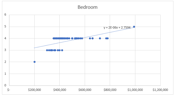
Figure 1: Association between number bedroom and property price
Figure 1 demonstrates the association between bedroom and property price. Though the plots did not showcase anything clearly, however, an upward sloping trend line demonstrated a positive association between the variables (Schober et al., 2018). Positive association demonstrates increase in number of bedrooms, increase the housing price.
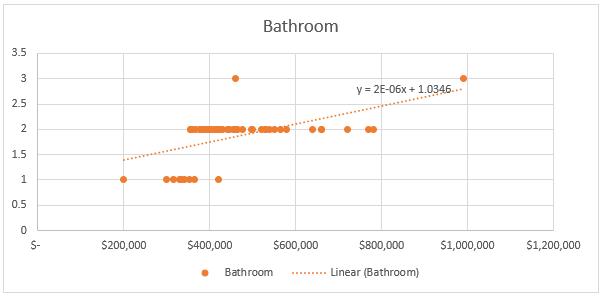
Figure 2: Association between bathroom number and property price
As per the figure 2 it can be seen that there is also an upward trend in price as the number of bathroom increases. Hence, the association is positive, however the degree of association is not clear from here.
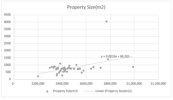
Figure 3: Association between property size and property price
Figure 3 demonstrated as the property size increase; price of property also increase. However, the plots are not scattered demonstrating, as the property size increase price of property does not increase moderately. Hence, though the trend line showcase a positive association between two values, yet the degree of association is not very high.
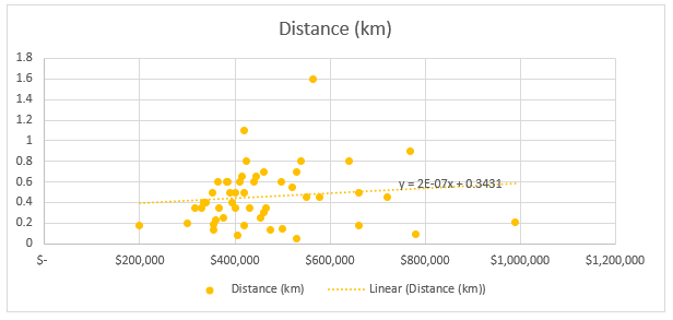
Figure 4: Association between distance from metro and property price
Figure 4 demonstrates a positive association between the distance from metro and property price. Hence, with rise in distance of property from metro, price tends to rise. However, as the distance increase, housing price does not increase proportionately as per plot demonstrating a weak association.
Task 3: Multiple regression:
To develop model that can predict the housing price based on independent variables, multiple regression has been done here. As per table 2 in appendix, following regression model can be mentioned:
Y = -169462.44 + 104230.45 * X1 + 80772.80 * X2 + 100.18 * X3 + 25196.60 * X4 [Where, Y is property price, X1 is bedroom number, X2 is bathroom number, X3 is property size and X4 is distance from metro]
Task 4: Slope coefficient interpretation:
As per table 2, slope coefficient of bedroom is 104230.45 which mean, change in 1 unit of bedroom can lead the property price to increase by $104230.45. Slope coefficient of bathroom demonstrates 1 unit of bathroom addition can lead to rise in house price by $80772.80. As per property size slope coefficient, 1 m2 rise in property size increase the property price by $100.18. Distance slope coefficient, 1 km rise in distance can increase the housing price by $25196.60.
Task 5: R2 and adjusted R2 model:
R square value of the model is 0.53, which mean independent variables can explain 53% of variability of the data in dependent variable. Adjusted R Square demonstrates how additional independent variable can change the predictability of the model for dependent variable (Sharma et al., 2021). Adjusted R Square value of 0.49, means addition of exploratory variables can actually fails to make the model more significant in predicting variability of data.
Task 6: Test of significance of model:
Null hypothesis: H0: Fit of intercept only model is equal to predicted model
Alternative hypothesis: H1: Fit of intercept only model is significantly reduced compared to predicted model
As per the ANOVA in table, F value is 0.00, which is lower than critical value of 0.05. Hence, the model is a good fit model and null hypothesis is accepted here.
Task 7: Test of significance of independent variable:
At 0.05 level of significance, as per table 2, only bedroom and property size seems to significantly influence the property price as their p value is 0.02 and 0.00 respectively. For other exploratory variables, p value is 0.1 (for bathroom) and 0.62 (for distance) which is higher than critical value of 0.05. Thus, bathroom and distance cannot significantly influence the property price.
Considering the significance of bedroom and property size, these factors can only be included in the regression model; thus, the revised regression model is as follows:
Y = -169462.44 + 104230.45 * X1 + 100.18 * X3
Task 8: 95% confidence interval of property size:
Confidence interval = b1 ± t(1-α)/2, n-2 * se(b1)
At 95% confidence interval, t(1-α)/2, n-2 = 2.011
b1 = 100.18
se(b1) = 28.92
Confidence interval = 100.18 ± 2.011 * 28.92 = 58.13
Confidence interval = 100.18 ± 58.13 = 158.13, 42.05
So, with 95% confidence interval, one m2 change in property size change the housing price between $158.13 and $42.05.
Task 9: 95% Confidence interval of distance:
Confidence interval = b1 ± t(1-α)/2, n-2 * se(b1)
At 95% confidence interval, t(1-α)/2, n-2 = 2.011
b1 = 25196.60
se(b1) = 51167.47
Confidence interval = 25196.60 ± 2.011 * 51167.47 = 128094.38, -77701.18
So, with 95% confidence interval it can be said that with 1 km change in distance, housing price change between $128094.38 and -$77701.18.
Task 10: Estimation of House Price:
House price at Clayton with 3-bedroom, 1 bathroom, 191 m2 property size and .5 km distance to metro:
Y = -169462.44 + 104230.45 * 3 + 100.18 * 191 = $162363.61
Hence, the estimated property price at Clayton would be $162363.31
Reference:

Download Samples PDF
Related Sample
- MBA652 Strategy and Leadership in Tourism and Hospitality Report 1
- BUSN20016 Research in Business Assignment
- MATH11247 Foundation Mathematics Assignment 2
- Engineering Strategy Assessment
- Finance Broking in Practice Assignment
- Recognitions Measurements and Disclosures of IAS 41
- TECH5300 Bitcoin Case Study 2
- BUMGT6958 Comparative Issues in International Management Essay 3
- BST904 Creativity Innovation and Enterprise Assignment
- BUMGT6973 Project Management Report 2
- HI6008 Business Research Project Report 1
- MBIS4010 Professional Practice in Information Systems Essay
- COMP1001 Data Communications and Networks Assignment
- MBA501 Dynamic Strategy and Disruptive Innovation Assignment
- MN623 Cyber Security and Analytics Assignment
- MBAS905 Advanced Business Analytics Case Study 1
- MKT101A Marketing Fundamentals Assignment
- MGT604 Strategic Management Report
- BUECO5903 Business Economics Assignment Part A
- BUECO5903 Assignment

Assignment Services
-
Assignment Writing
-
Academic Writing Services
- HND Assignment Help
- SPSS Assignment Help
- College Assignment Help
- Writing Assignment for University
- Urgent Assignment Help
- Architecture Assignment Help
- Total Assignment Help
- All Assignment Help
- My Assignment Help
- Student Assignment Help
- Instant Assignment Help
- Cheap Assignment Help
- Global Assignment Help
- Write My Assignment
- Do My Assignment
- Solve My Assignment
- Make My Assignment
- Pay for Assignment Help
-
Management
- Management Assignment Help
- Business Management Assignment Help
- Financial Management Assignment Help
- Project Management Assignment Help
- Supply Chain Management Assignment Help
- Operations Management Assignment Help
- Risk Management Assignment Help
- Strategic Management Assignment Help
- Logistics Management Assignment Help
- Global Business Strategy Assignment Help
- Consumer Behavior Assignment Help
- MBA Assignment Help
- Portfolio Management Assignment Help
- Change Management Assignment Help
- Hospitality Management Assignment Help
- Healthcare Management Assignment Help
- Investment Management Assignment Help
- Market Analysis Assignment Help
- Corporate Strategy Assignment Help
- Conflict Management Assignment Help
- Marketing Management Assignment Help
- Strategic Marketing Assignment Help
- CRM Assignment Help
- Marketing Research Assignment Help
- Human Resource Assignment Help
- Business Assignment Help
- Business Development Assignment Help
- Business Statistics Assignment Help
- Business Ethics Assignment Help
- 4p of Marketing Assignment Help
- Pricing Strategy Assignment Help
- Nursing
-
Finance
- Finance Assignment Help
- Do My Finance Assignment For Me
- Financial Accounting Assignment Help
- Behavioral Finance Assignment Help
- Finance Planning Assignment Help
- Personal Finance Assignment Help
- Financial Services Assignment Help
- Forex Assignment Help
- Financial Statement Analysis Assignment Help
- Capital Budgeting Assignment Help
- Financial Reporting Assignment Help
- International Finance Assignment Help
- Business Finance Assignment Help
- Corporate Finance Assignment Help
-
Accounting
- Accounting Assignment Help
- Managerial Accounting Assignment Help
- Taxation Accounting Assignment Help
- Perdisco Assignment Help
- Solve My Accounting Paper
- Business Accounting Assignment Help
- Cost Accounting Assignment Help
- Taxation Assignment Help
- Activity Based Accounting Assignment Help
- Tax Accounting Assignment Help
- Financial Accounting Theory Assignment Help
-
Computer Science and IT
- Operating System Assignment Help
- Data mining Assignment Help
- Robotics Assignment Help
- Computer Network Assignment Help
- Database Assignment Help
- IT Management Assignment Help
- Network Topology Assignment Help
- Data Structure Assignment Help
- Business Intelligence Assignment Help
- Data Flow Diagram Assignment Help
- UML Diagram Assignment Help
- R Studio Assignment Help
-
Law
- Law Assignment Help
- Business Law Assignment Help
- Contract Law Assignment Help
- Tort Law Assignment Help
- Social Media Law Assignment Help
- Criminal Law Assignment Help
- Employment Law Assignment Help
- Taxation Law Assignment Help
- Commercial Law Assignment Help
- Constitutional Law Assignment Help
- Corporate Governance Law Assignment Help
- Environmental Law Assignment Help
- Criminology Assignment Help
- Company Law Assignment Help
- Human Rights Law Assignment Help
- Evidence Law Assignment Help
- Administrative Law Assignment Help
- Enterprise Law Assignment Help
- Migration Law Assignment Help
- Communication Law Assignment Help
- Law and Ethics Assignment Help
- Consumer Law Assignment Help
- Science
- Biology
- Engineering
-
Humanities
- Humanities Assignment Help
- Sociology Assignment Help
- Philosophy Assignment Help
- English Assignment Help
- Geography Assignment Help
- Agroecology Assignment Help
- Psychology Assignment Help
- Social Science Assignment Help
- Public Relations Assignment Help
- Political Science Assignment Help
- Mass Communication Assignment Help
- History Assignment Help
- Cookery Assignment Help
- Auditing
- Mathematics
-
Economics
- Economics Assignment Help
- Managerial Economics Assignment Help
- Econometrics Assignment Help
- Microeconomics Assignment Help
- Business Economics Assignment Help
- Marketing Plan Assignment Help
- Demand Supply Assignment Help
- Comparative Analysis Assignment Help
- Health Economics Assignment Help
- Macroeconomics Assignment Help
- Political Economics Assignment Help
- International Economics Assignments Help
-
Academic Writing Services
-
Essay Writing
- Essay Help
- Essay Writing Help
- Essay Help Online
- Online Custom Essay Help
- Descriptive Essay Help
- Help With MBA Essays
- Essay Writing Service
- Essay Writer For Australia
- Essay Outline Help
- illustration Essay Help
- Response Essay Writing Help
- Professional Essay Writers
- Custom Essay Help
- English Essay Writing Help
- Essay Homework Help
- Literature Essay Help
- Scholarship Essay Help
- Research Essay Help
- History Essay Help
- MBA Essay Help
- Plagiarism Free Essays
- Writing Essay Papers
- Write My Essay Help
- Need Help Writing Essay
- Help Writing Scholarship Essay
- Help Writing a Narrative Essay
- Best Essay Writing Service Canada
-
Dissertation
- Biology Dissertation Help
- Academic Dissertation Help
- Nursing Dissertation Help
- Dissertation Help Online
- MATLAB Dissertation Help
- Doctoral Dissertation Help
- Geography Dissertation Help
- Architecture Dissertation Help
- Statistics Dissertation Help
- Sociology Dissertation Help
- English Dissertation Help
- Law Dissertation Help
- Dissertation Proofreading Services
- Cheap Dissertation Help
- Dissertation Writing Help
- Marketing Dissertation Help
- Programming
-
Case Study
- Write Case Study For Me
- Business Law Case Study Help
- Civil Law Case Study Help
- Marketing Case Study Help
- Nursing Case Study Help
- Case Study Writing Services
- History Case Study help
- Amazon Case Study Help
- Apple Case Study Help
- Case Study Assignment Help
- ZARA Case Study Assignment Help
- IKEA Case Study Assignment Help
- Zappos Case Study Assignment Help
- Tesla Case Study Assignment Help
- Flipkart Case Study Assignment Help
- Contract Law Case Study Assignments Help
- Business Ethics Case Study Assignment Help
- Nike SWOT Analysis Case Study Assignment Help
- Coursework
- Thesis Writing
- CDR
- Research

.png)
~5.png)
.png)
~1.png)


.png)