Sample SIT741 Statistical Data Analysis Assignment

SIT741 Statistical Data Analysis Assignment Sample

Q1: Car accident dataset (10 points)

Q1.1: How many rows and columns are in the data? Provide the output from your R Studio

Q1.1: What data types are in the data? Use data type selection tree and provide detailed explanation. (2 points for data types, 2 points for explanation)

Q1.3: How many regions are in the data? What time period does the data cover? Provide the output from your R Studio

Q1.4: What do the variables FATAL and SERIOUS represent? What’s the difference between them?

Q2: Tidy Data

Q2.1 Cleaning up columns. You may notice that the road traffic accidents csv file has two rows of heading. This is quite common in data generated by BI reporting tools. Let’s clean up the column names. Use the code below and print out a list of regions in the data set.

Q2.2 Tidying data

a) Now we have a data frame. Answer the following questions for this data frame.

- Does each variable have its own column? (1 point)

- Does each observation have its own row? (1 point)

- Does each value have its own cell? (1 point)

b) Use spreading and/or gathering (or their pivot_wider and pivot_longer new equivalents) to transform the data frame into tidy data. The key is to put data from the same measurement source in a column and to put each observation in a row. Then, answer the following questions.

I. How many spreading (or pivot_wider) operations do you need?

II. How many gathering (or pivot_longer) operations do you need?

III. Explain the steps in detail.

IV. Provide/print the head of the dataset.

c) Are the variables having the expected variable types in R? Clean up the data types and print the head of the dataset.

d) Are there any missing values? Fix the missing data. Justify your actions.

Q3: Fitting Distributions

In this question, we will fit a couple of distributions to the “TOTAL_ACCIDENTS” data.

Q3.1: Fit a Poisson distribution and a negative binomial distribution on TOTAL_ACCIDENTS. You may use functions provided by the package fitdistrplus.

Q3.2: Compare the log-likelihood of two fitted distributions. Which distribution fits the data better? Why?

Q3.3 (Research Question): Try one more distribution. Try to fit all 3 distributions to two different accident types. Combine your results in the table below, analyse and explain the results with a short report.

Q4: Source Weather Data

Above you have processed data for the road accidents of different types in a given region of Victoria. We still need to find local weather data from the same period. You are encouraged to find weather data online.

Besides the NOAA data, you may also use data from the Bureau of Meteorology historical weather observations and statistics. (The NOAA Climate Data might be easier to process, also a full list of weather stations is provided here: https://www.ncei.noaa.gov/pub/data/ghcn/daily/ghcnd-stations.txt )

Answer the following questions:

Q4.1: Which data source do you plan to use? Justify your decision. (4 points)

Q4.2: From the data source identified, download daily temperature and precipitation data for the region during the relevant time period. (Hint: If you download data from NOAA https://www.ncdc.noaa.gov/cdo-web/, you need to request an NOAA web service token for accessing
the data.)

Q4.3: Answer the following questions (Provide the output from your R Studio):

- How many rows are in your local weather data?

- What time period does the data cover?

Q5 Heatwaves, Precipitation and Road Traffic Accidents

The connection between weather and the road traffic accidents is widely reported. In this task, you will try to measure the heatwave and assess its impact on the road accident statistics. Accordingly, you will be using the car_accidents_victoria dataset together with the local weather data.

Q5.1. John Nairn and Robert Fawcett from the Australian Bureau of Meteorology have proposed a measure for the heatwave, called the excess heat factor (EHF). Read the following article and summarise your understanding in terms of the definition of the EHF. https://dx.doi.org/10.3390%2Fijerph120100227

Q5.2: Use the NOAA data to calculate the daily EHF values for the area you chose during the relevant time period. Plot the daily EHF values.

Q6: Model Planning

Careful planning is essential for a successful modelling effort. Please answer the following planning questions.

Q6.1. Model planning:

a) What is the main goal of your model, how it will be used?

b) How it will be relevant to the emergency services demand?

c) Who are the potential users of your model?

Q6.2. Relationship and data:

a) What relationship do you plan to model or what do you want to predict?

b) What is the response variable?

c) What are the predictor variables?

d) Will the variables in your model be routinely collected and made available soon enough for prediction?

e) As you are likely to build your model on historical data, will the data in the future have similar characteristics?

Q6.3. What statistical method(s) will be applied to generate the model? Why?

Q7: Model The Number of Road Traffic Accidents

In this question you will build a model to predict the number of road traffic accidents. You will use the car_accidents_victoria dataset and the weather data. We can start with simple models and gradually makemthem more complex and improve them. For example, you can use the EHF as an additional predictor to augment the model. Let’s denote by Y the road traffic accident variable.

Randomly pick a region from the road traffic accidents data.

Q7.1 Which region do you pick?

Q7.2 Fit a linear model for Y according to your model(s) above. Plot the fitted values and the residuals. Assess the model fit. Is a linear function sufficient for modelling the trend of Y? Support your conclusion with plots.

Q7.3 As we are not interested in the trend itself, relax the linearity assumption by fitting a generalised additive model (GAM). Assess the model fit. Do you see patterns in the residuals indicating insufficient model fit?

Q7.4 Compare the models using the Akaike information criterion (AIC). Report the best-fitted model through coefficient estimates and/or plots.

Q7.5 Analyse the residuals. Do you see any correlation patterns among the residuals?

Q7.6 Does the predictor EHF improve the model fit?

Q7.7 Is EHF a good predictor for road traffic accidents? Can you think of extra weather features that may be more predictive of road traffic accident numbers? Try incorporating your feature into the model and see if it improves the model fit. Use AIC to prove your point.

Q8: Reflection

In the form of a short report answer the following questions (no more than 3 pages for all questions):

Q8.1: We used some historical data to fit regression models. What additional data could be used to improve your model?

Q8.2: Overall, have your analyses answered the objective/question that you set out to answer?

Q8.3: Missing value [10 marks]. If the data had some with missing values, what methods would you use to address this issue? (Provide 1-3 relevant references)

Q8.4. Overfitting [10 marks]. In Q7.4 we used the Akaike information criterion (AIC) to compare the models. How would you tackle the overfitting problem in terms of the number of explanatory variables that you could face in building the model? (Provide 1-3 relevant references)

Solution

Q1. Car Accident Dataset

Q1.1 Dataset description

Figure 1: Dimension of Dataset
(Source: R Studio)

The Dataset contains 1644 Rows and 29 Columns which are generated using the “dim” code.

Q1.2 Data type identification

Figure 2: Type of Dataset
(Source: R Studio)

The Dataset is based on the character datatype which means every data in the dataset contains one byte character.

Figure 3: Selection Tree Code
(Source: R Studio)

The code sets each column of the `car_accidents” dataset and identifies and prints the data type of each column used in this dataset. The type function for The Assignment Helpline determines whether the column is of “numeric”, “character”, “factor” or “date” and returns the type. It has proved to be useful for the identification of the structure of the datasets necessary for further steps of data preprocessing and analysis in the research.

Q1.3 Identification of the regions in dataset

Figure 4: Number of Regions
(Source: R Studio)

In the Dataset, there are a total of 7 regions available which are generated using the given codes.

Figure 5: Date Range
(Source: R Studio)

The Dataset covers the date range between 1st January 2016 to 30th June 2020.

Q1.4 Representation of FATAL and SERIOUS variables

The variables FATAL and SERIOUS are measures of the number of road traffic accidents by area of the world in which they occurred. FATAL shows the total, fatal pedestrian accidents and SERIOUS, indicates the number of severe, but not fatal, injuries. The critical difference lies in the outcome: fatalities refer to loss of lives while serious injuries point towards possible long-term health complications (Jiang et al. 2024). This is particularly important in terms of evaluation of the level of acuity and hence, of resource use in emergency services treatment.

Q2. Tidy Data

Q2.1 Cleaning up columns.

Figure 6: Cleaning up Columns
(Source: R Studio)

The code removes some unwanted characters and spaces from the column names of car accident data which are available in the car_accidents_victoria.csv file data set, In this file there are two rows of headers. The first two rows are read separately, various double underscores are used to generate different names for the columns, and the number ‘0’ is added to certain columns. The column named daily_acccidents is then taken from the cleaned dataset after omitting the first two rows of the Excel file and the column headers are given standard names for further use. This makes certain data manipulation to be correct and makes subsequent modelling to be clear.

Q2.2 Tidying data

a

Figure 7: Column Identification
(Source: R Studio)

The code then demonstrates whether each variable in the daily_accidents dataset is properly indexed in its column by using the is.atomic function. The output reproduced this with the value of `TRUE’ signifying that the data was well formatted for analysis.

Figure 7: Row Identification
(Source: R Studio)

The code guarantees each observation in the daily_accidents has its row by way of checking to ensure no rows are repeated in the dataset while also ensuring the DATE column does not hold any missing values. The TRUE output as shown below also accredits the correct structuring of the data for analysis.

Figure 8: Cell Identification
(Source: R Studio)

It also confirms that each value in the daily_accidents dataset has its row by using is.na() to test that no value in this dataset is missing. To output FALSE, there is likely an information quality problem which is always common with data, that makes them improper for further analysis.

b

i)

Figure 9: Pivot Wider
(Source: R Studio)

A single `pivot_wider` transformation process is required to keep reshaping the dataset by widening different types of accidents, namely the accident type (FATAL, SERIOUS), which has to be categorized distinctly for every observation.

ii)

Figure 10; Pivot Longer
(Source: R Studio)

To merge multiple region-based columns into a single spread column while ensuring that all are under one variable to return the data to their tidy shape a double `pivot_longer` is needed.

iii)

The code begins with the `pivot_longer` function to transform multiple region-specific accident columns into one single column called `Region` which subsumes the types of accidents (FATAL, SERIOUS) under the column title `Accident_Type`. The `names_pattern` argument inputs the substring `Region` and `Accident_Type` out of column names because their matching is assumed to be most precise in the usage of regular expressions. Then the resulting long-format data is processed using `pivot_wider` and `Accident_Type` values are turned into variables. This extends the row of columns horizontally so that each type of accident is separated by its column, thus simplifying analysis between areas. The last `tidy_data’ format is convenient for the further analysis and modelling phase, visualisation and other statistical techniques (Pereira et al. 2019).

iv)

Figure 11: Head of Data
(Source: R Studio)

The code reshapes the ‘daily_accidents’ dataset so that it has a tidy form. The `long_data’ shows the same accident data as in the previous exercise but this data is in a long format with columns Region, Accident_Type, and their values. The `tidy_data` format then broadens these accident types into individual columns to make a clearer structure for counting accidents within regions over time.

c

Figure 12: Head Data
(Source: R Studio)

The various variables in the dataset might not be initially or automatically read in the expected form, for example, `DATE` may be read as a character `Date`(s), or accident counts as characters. For data type correction, there is a need to transform DATE to Date type while accident columns to numeric form of data. This improves the analysis of the data and also prevents a mistake made during data modelling from going unnoticed.

d

Yes, there are many cases of missing values in the dataset that lead to distortion of results. It is better to use the median or something called forwards filling because trends are weighed in such cases and they do not mislead in case some values are missing.

Q3. Fitting Distribution

Q3.1 Poisson distribution and a negative binomial distribution

Figure 13: Poisson Distribution
(Source: R Studio)

Poisson & Negative binomial distributions are then fitted on the `TOTAL_ACCIDENTS’ variable using the ‘fitdistrplus’ package. It can summarise and plot both models for easy comparison of goodness of distribution fit. This helps in its estimation to know which model best suits the prediction of variation in the accident count.

Q3.2 Comparison of the log-likelihood

Figure 14: LogLikelihood
(Source: R Studio)

The Negative Binomial model again is found to have a better fit with the data as its log-likelihood (-179060.2) is higher than that of Poisson ( -186547.4) while its AIC ( 358124.4) and BIC ( 358141.8) are comparatively lower to that of Poisson. This implies improved data modelling because the uncertainty in measurement is preserved as will be discussed later.

Q3.3 Research Question

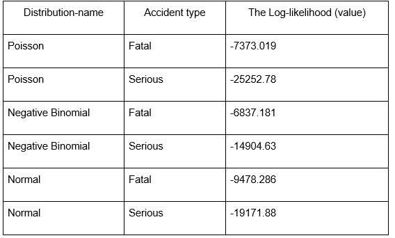
Table 1: Poisson Distribution
(Source: Self-Created)

According to the results, the Negative Binomial distribution has more log-likelihood values for Fatal and Serious types among all the analysed models, which means they are adjusted better than Poisson and Normal distributions. Negative Binomial is more appropriate where the variability of variance is high such as in accident modelling. The Poor fit of Poisson distribution indicates that it is inefficient for capturing the variability of the data, majority while the Moderate fit of the Normal distribution to the current data shows it is imprecise in estimation of count-based accident data. Therefore, the Negative Binomial model is suitable for this dataset in particular because of the effectiveness of its estimation in the case of overdispersion.

Q.4: Source Weather Data

Q.4.1 Data source justification

The historical weather observation data from the Bureau of Meteorology is chosen for its rich and accurate record of the environmental data, which is necessary for estimating the correlation between different weather conditions and traffic crash rates on the roads.

Q.4.2 Downloading dataset

Figure 14: Downloaded Dataset
(Source: EXCEL)

The Dataset is downloaded from the Bureau of Meteorology website.

Q.4.3 Answer the following questions (Provide the output from your R Studio):

Figure 15: Rows Identification
(Source: R Studio)

In the dataset there are 26115 rows are available.

Figure 16: Time Period
(Source: R Studio)

Time period is covered within 1st January 2016 to 30th December 2016.

Q.5: Heatwaves, precipitation and road traffic accidents

Q5.1 Summarization of the understanding

The Excess Heat Factor (EHF) measures heatwave intensity by analysing short-term and long-term heat anomalies. It compares the 30-day average to a three-day mean daily temperature above the 95th percentile. A high EHF indicates a severe heatwave, indicating health and environmental damage.

Q.5.2 Calculate the daily EHF values

Figure 17: EHF Factor
(Source: R Studio)

The graph shows January 2016–January 2017 daily Excess Heat Factor (EHF) data. The highest heat intensity was in April 2016. Summer EHF spikes are more frequent and intense, indicating heat stress. Heatwave severity decreases during cooler seasons.

Q.6: Model planning

Q.6.1 Model planning:

a)

The main goal is to predict road accidents using meteorological data for proactive traffic management and safety planning.

b)

Emergency services can disperse resources and reduce response times by predicting accident hotspots with the model.

c)

Traffic management, emergency services, urban planners, insurance companies, and public safety agencies can use it to improve road safety and resource allocation.

Q.6.2 Relationship and data

a)

Meteorological parameters like temperature, humidity, and EHF are linked to road accidents in different regions by the model. Accident probability and intensity are predicted based on meteorological conditions to aid prevention and resource allocation.

b)

Number of Road Accident will be the Response Variable from the car accident dataset.

c)

Temperature (temp), Humidity (humid), and Excess Heat Factor (EHF) are predictor variable from weather dataset

d)

Meteorological authorities collect and modify temperature, humidity, and EHF in real time to ensure accurate road accident predictions.

e)

In the absence of significant climatic alterations, meteorological patterns and vehicular accident trends are expected to adhere to seasonal fluctuations, rendering the model relevant for future forecasts.

Q.6.3 Application of the statistical model

Linear Regression will be employed for trend analysis, whereas Generalised Additive Models (GAM) will be utilised for non-linear relationships between weather and accident frequency. These methods enable the representation of smooth functions for variables such as temperature and humidity, which may not influence accidents linearly, to elucidate complex interconnections and improve forecasting precision.

Q.7 Model the Number of Road Traffic Accidents

Q.7.1 Region selection

Western Region is selected for the modelling.

Q.7.2 Fitting linear model

Figure 18: Linear Model
(Source: R Studio)

This graph compares the number of accidents in the WESTERN region (blue lines) to the linear model's predictions (red line). Despite increases in accident numbers, the linear model remains constant, failing to capture these oscillations. It appears that a linear model cannot accurately capture road accident trends. Systematic patterns in the residuals plot suggest that a Generalised Additive Model (GAM) might be better at capturing non-linear interactions. By showing that complex models improve predictions, this influences research.

Q.7.3 Fitting a generalised additive model

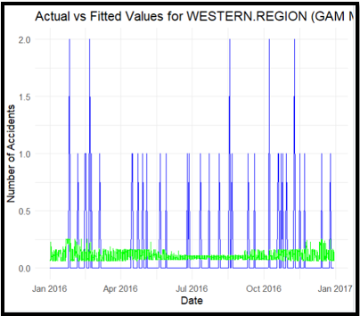
Figure 19: GAM Model
(Source: R Studio)

The graph illustrates the actual accident numbers (blue lines) in comparison to the fitted values using the GAM model (green line) for the WESTERN area. In contrast to the linear model, the GAM model accounts for local changes in accident patterns, demonstrating a superior match. Nonetheless, the increases in actual incidents remain inadequately reflected, indicating persistent patterns and possible underfitting. This suggests that the adaptable GAM is unable to properly encapsulate the non-linearities inherent in accident data, underscoring the necessity for more sophisticated models, including interaction terms or seasonal components.

Q.7.4 Comparison of the models

Figure 20: Comparison
(Source: R Studio)

AIC data show that the GAM model (AIC = 19103.07) matches better than the linear model (AIC = 19362.41). Non-linear patterns are better captured by the GAM model than the linear approach. GAM is better for accident analysis forecasts because meteorological variables and accident incidences are interconnected.

Q.7.5 Residual analysis

The GAM model residuals show patterns, indicating correlation. Clusters or patterns in residuals suggest model neglect of variability. Model efficacy may decrease due to time dependencies or omitted factors. This highlights the need for more advanced methods, such as time-series elements, to accurately depict accident dynamics and improve predictive precision.

Q7.6 Improvisation of predictor EHF

EHF quantifies the impact of severe heat on accident frequency, enhancing model fit and precision.

Q.7.7 Evaluation of EHF

EHF serves as a reliable predictor, as excessive heat can influence driver behaviour and vehicle performance, resulting in accidents. Nevertheless, supplementary meteorological variables such as precipitation, wind velocity, and visibility may possess greater forecasting capability. For example, precipitation can enhance road slipperiness, yet reduced sight can hinder driver reaction time. Incorporating precipitation into the model in conjunction with EHF allows us to evaluate whether it enhances model performance. An increase in model fit is suggested by a decrease in AIC with the inclusion of precipitation. This modification facilitates the capturing of a broader spectrum of meteorological factors impacting road safety, hence rendering the model more comprehensive for accident prediction.

Q.8 Reflection

Q.8.1 Recommendation of data

Additional data, including traffic density, road conditions, vehicle classifications, driver demographics, and accident severity, could substantially improve the model. Incorporating these characteristics would enhance the comprehension of accident causation, hence augmenting predictive efficacy and precision.

Q.8.2 Justification of the fulfilment of the research objectives

Indeed, my investigations have partially fulfilled the purpose by identifying critical meteorological variables influencing road accidents. Nevertheless, the models exhibit certain limits, suggesting that the inclusion of supplementary parameters could enhance prediction accuracy and reliability.

Q.8.3 Missing Value

In the presence of missing values, I would employ techniques such as mean or median imputed to provide continuous variables, mode imputation for categorical variables, or more sophisticated algorithms like KNN imputation and multiple imputation to maintain data integrity (Lee a& Yun, 2024).

Q.8.4 Overfitting

To address overfitting, I would employ approaches such as stepwise selection, regularisation methods (LASSO or Ridge regression), and cross-validation to minimise the number of explanatory variables, preserving just the most important predictors to enhance model generalisability (Laufer et al. 2023).  

References