Sample STAT6003 Statistics for Financial Decisions Assignment

STAT6003 Statistics for Financial Decisions Assignment Sample

Task 1:

Selecting your Random Sample and Creating your Sample Data File ( 8 Marks)

In order to select the sample data that will form the basis of your assignment you will need to make use of the random number table provided with this assignment help. The provided table of random numbers is, as the title suggests, a sequence of randomly generated numerical digits (0 to 9). These digits are arranged in a table with one hundred rows numbered 01 to 00 and twenty columns spread over two pages. The entries in each column of each row consist of five single digits.

The property data from which you will select your sample data consists of 400 IDs each with an identifying property number (PN) ranging from 1 (or 001) to 400.

Your first task is to select 50 three digit random (property) numbers ranging from 001 to 400 from the provided table of random numbers. We will ask you to select 50 numbers, to begin with, just to cover the distinct possibility that you may select the same three digit number more than once. The type of simple random sampling that we will be engaged in here is termed “without replacement” because we specifically do not want to allow a property identification number to be selected more than once.

In order to select your 50 random property identification numbers you will need to first go to a starting position row and column in the random number table. Defined by the last three digits of your Torrens University student identification number. The last two digits of your Torrens ID number identifies the row and the third last digit identifies the column of your (relatively) “unique” starting position. For the demonstration last three digits of 312, reading across row 12 from left to right starting at column 3 as instructed, you would encounter the following three digit numbers; 293 313 381 349 656 985 295

You need to record these first three acceptable ID numbers, 293, 313, 381 and 349 into the first column of an Excel spread-sheet and then continue this process until fifty valid three-digit personal identification numbers selected.

Task 2:

1. Provide the complete summary statistics for Market Price ($000) and Age of house (years). (5 Marks)

2. Describe the shape of the distributions for Market Price ($000) and Age of house (years). (5 Marks)

3. Test whether the population’s average Market Price ($000) is different from 777. (5 Marks)

4. Construct a 95% confidence interval for the Market Price ($000), also Interpret the confidence interval. (4 Marks)

5. Provide an introduction section on the rationale of your model , sample size, and the dependent and independent variables (including their unit of measurement) in this model. (4 Marks)

6. Plotthe dependent variable against each independent variable using scatter plot/dotfunction in Excel. Examine these scatter plots and correctly assess the strength and the nature of the
relationship between the dependent and the independent variables? (6 Marks)

7. Present the multiple regression model with complete regression summary output in your assignment. (6 Marks)

8. Provide the simple linear regression data analysis for the market price as the response variable and the Land size in Square meters as the explanatory variable. Write down the least square regression equation and correctly interpret the equation. (6 Marks)

9. Write a clear interpretation of the slope of the regression line from question 8. You must refer to the variables of interest. (4 Marks)

10. What is the value of the coefficient of determination for the relationship between the dependent and independent variable from question 8. Interpret this value accurately and ina meaningful way. (4 Marks)

11. State the 95% confidence interval for the slope coefficient and interpret this interval from question 8. (5 Marks)

12. Compare the multiple regression model (question 7) and simple linear regression model (question 8) and evaluate the goodness of fit between these two modelling techniques.(8 Marks)

13. Predict the market price of a house (in $) with a building area of 300 square meters. Explain why your answer is valid.(4 Marks)

14. By performing an appropriate hypothesis test what decision and conclusion would you draw about the hypothesis that the Land size in Square meters useful in predicting the market price of a house (in $)? Use the data provided to justify your answer, as appropriate.When answering this research question. (8 Marks)

15. For statistical analysis involving hypothesis testing in this assignment, you are required to:
• Formulate the null and alternative hypotheses for full model.
• State your statistical decision using significant value (α) of 5% for this test.
• State your conclusion in this context.

SOLUTION

Summary statistics is used to summarise data and get information from it. The summary statistics table comprises the values of central tendency which are obtained in the form of mean, median and mode along with measures of dispersion is obtained in the form of standard deviation and sample variance. In addition to this, distribution of data can be understood by calculating skewness, kurtosis and range (Cooksey 2020). Hence, from this table one can understand where the mean lies and how data is distributed around the mean value. The summary statistics of market price ($000) is shown in table 1. Similarly, the summary statistics of age of house that is measured in years is shown in table 2.

Table 1: Summary Statistics of Market Price ($000):

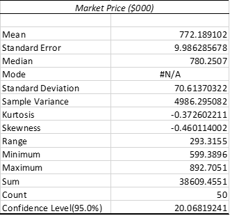
From the table, it is observed that average market price is $772.19 (‘000). Moreover, the standard deviation is 70.61 which implies that market prices of houses do not deviate largely from the mean value. The minimum market price of house in the collected sample file is $599.39 (‘000). Moreover, the maximum market price of house in the collected sample file is $ 892.71(‘000).

Table 2: Summary Statistics of Age of house (years)

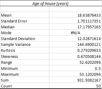
From the table, it is observed that average age of house is 18.63 years. Moreover, the standard deviation is 12.03 which implies that age of houses deviates largely from the mean value. The minimum age of house in the collected sample file is 0.5 year. Moreover, the maximum age of house in the collected sample file is 53.12 years.

2.

In statistics, skewness measures how a data set is distributed. A data set can be either symmetric or symmetric in nature. The main reason of measuring skewness is that it informs whether ata has larger extreme values or lower extreme values. As per the “Rule of Thumbs”, the skewness varies between -0.5 to 0.5 is known as symmetrical (Orcan 2020). The skewness of Market Price ($000) is -0.46 which lies within the boundary. Hence, it indicates that the distributions for this variable is almost symmetric. The shape of the distribution is also called a bimodal distribution.

On the other side, the skewness of Age of house (years) is 0.67 which lies between 0.5 and 1. Hence, it indicates that the distribution of data is moderately skewed towards the right direction. In other words, the distribution is positively skewed where mean value is higher than median.
The distributions of Market Price ($000) data as well as the same for Age of house (years) are demonstrated below by histograms.

 

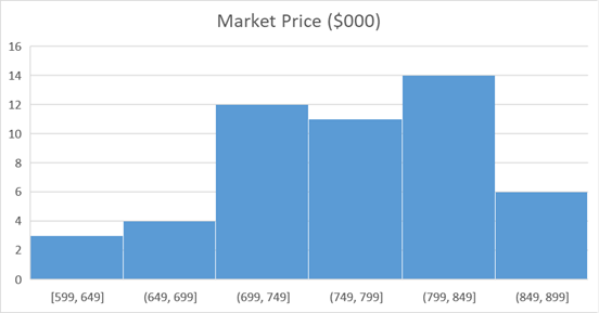
Figure 1: Distribution of Market Price ($000)

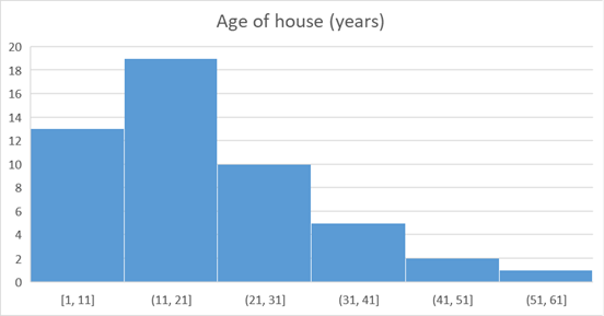
Figure 2: Distribution of Age of house (years)

3.

To understand if the average Market Price ($’000) of target population differs from 777 or not, one sample t-test (two-tailed) is conducted. Here, n is 50. However, population standard deviation is unknown. Hence, z-test cannot be applied.

Here, average Market Price ($ ‘000) is µ

Therefore, the null hypothesis is:

H0: the average Market Price ($’000) of the population is equal to 777
µ = 777
The alternative hypothesis is:
H1: the average Market Price ($’000) of target population is different from 777
µ ≠ 777
The outcome obtained from MS Excel is:

Table 3: One sample t-test (two-tailed test)

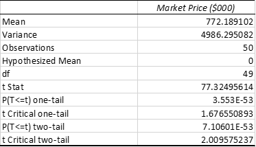
Here, the t statistics is 77.32 which is higher than t Critical two-tail value, which is 2. Hence, here, the null hypothesis is rejected. Moreover, the P-value in two-tail test is 0.00 which is less than 0.05 at 5% significance level (Xu et al. 2017). Hence, again the null-hypothesis is rejected. Thus, it implies that average Market Price ($’000) of the target population is not equal to 777.

4.

As per the outcome obtained from Excel, the value of Confidence Level at 95% is 20.07
Thus, the lower interval is (mean – confidence level) = 752.12
the upper interval is (mean + confidence level) = 792.26
Here, confidence interval represents actual upper and lower values. It implies that the 95% of the time, the researcher can expect that the real mean will fall between 752.12 and 792.26.

5.

The model of regression analysis is selected to forecast the dependent variable by independent variable(s). The regression model is categorised depending on the number of independent variables. Hence, to determine dependent variable with one independent variable, linear regression model is applied. Moreover, to determine dependent variable with more than one independent variable, multiple regression model is applied (Montgomery, Peck and Vining 2021). The sample size in this study is 50, which are selected by applying simple random sampling technique without replacement. The four variables are market price ($000), Sydney price Index, total number of square meters and age of house (years). In regression model, market price ($000) is considered as dependent variable while others are considered as independent variables. The scatter plots are also made to measure the strength of association between independent and dependent variable.

6.

A scatter plot is a form of statistical diagram that shows values for two variables and measure a relationship between them. Hence, this plot is used to show the relationship visually to understand the strength type of the relationship between these two variables. In general, this plot is of 3 types, which are positive, negative and no correlation (Akoglu 2018). The relationship of the dependent variable with each independent variable is shown by scatter plots.

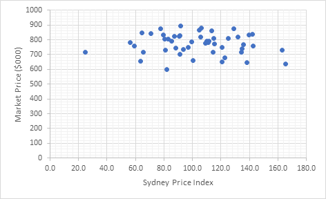
Figure 3: Scatter Plot Diagram between Sydney Price Index and Market Price ($000)

Figure 3 represents a scatter plot diagram to show relationship between independent variable Sydney Price Index and dependent variable Market Price ($000). From the figure, it is seen that these two variables do not have any relationship with each other. In other words, the diagram indicates that Sydney Price Index does not relate with Market Price ($000). Hence, variation in Sydney Price Index cannot tend the Market price to variation in same or opposite direction specifically.
 

Figure 4: Scatter Plot Diagram between Total number of square meters and Market Price ($000)

Figure 4 represents a scatter plot diagram to show relationship between independent variable Total number of square meters and dependent variable Market Price ($000). From the figure, it is seen that these two variables have strong and positive correlation. In other words, the diagram indicates that there if Sydney Price Index increases, Market Price ($000) price also increases and vice versa.

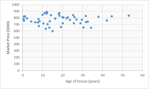
Figure 5: Scatter Plot Diagram between Age of house (years) and Market Price ($000)

Figure 5 represents a scatter plot diagram to show relationship between independent variable Age of house (years) and dependent variable Market Price ($000). From the figure, it is seen that these two variables do not have any relationship with each other. In other words, the diagram indicates that there is no relationship between Age of house (years) and Market Price ($000). Hence, age of house cannot tend the Market price to change in same or opposite direction specifically.

7.

The following table represents summary outcome of multiple regression model:

Table 4: Calculation of Multiple Regression

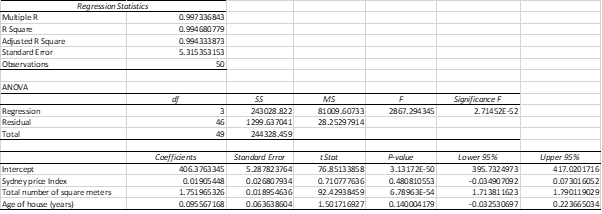
From table 4, the following equation of multiple regression is obtained:
Market Price ($000) = 406.38 + 0.02 Sydney Price Index + 1.75 Total number of square meters + 0.1 Age of house (years)

In this equation, 406.38 is the intercept of regression equation. Moreover, 0.02, 1.75 and 0.1 are beta coefficients. Beta coefficient of an independent variable implies the magnitude of change in the dependent variable when this independent variable changes by 1 unit.

If Sydney price index increases by 1%, the market price of houses will increase by $ 0.02 (‘000). If total number of land size increases by 1,75 square meters, then market price of house will increase by $1.75 (‘000). If age of houses increases by 1year, then market price of that house will increase by $0.1 (‘000). Hence, from the equation, it is seen that each independent variable has positive influence on the market price of house.

8.

Table 5: Calculation of Simple Linear Regression

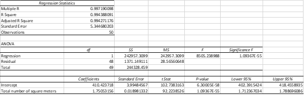
The obtained Simple linear regression equation is:
Market Price ($000) = 410.42 + 1.75 total number of square meters
According to the above equation, market price of a house can be high even if land size in square meters of the house is unavailable.

9.

From the multiple regression equation of question 8, the slopes are described below.
The slope of the regression line is the beta coefficient of total number of square meters. It implies that if land size increases by 1 square meters, the market price will increase by $1.75 (‘000).

10.

The value of R-square is 0.99 which means independent variable can define 99% of variation of the dependent variable.

11.

At 95% confidence interval, the slope coefficients are: lower limit: 1.712 and upper limit: 1.789. For intercept, the lower limit is 402.392 and upper limit is 418.456.

12.

The value of R-square in question 7 is 0.99 while that in question 8 is 0.9 as well. Hence, it is observed that the value of R-square in both models are almost equal to 1. Moreover, the value of the coefficient of determination or adjusted R-square for the association between dependent and autonomous variables is 0.99 as per table 4. It implies that independent variables can predict almost 99% of variation of the dependent variable. Hence, it indicates a strong and positive correlation between dependent and independent variables.
Hence, models fit the data perfectly.

13.

From simple linear regression equation, obtained in question 8, the market price of house (in $) can be obtained when a building is given as 300 square meters.

Market Price ($) = 410.42 + 1.75 * 300
Market Price ($) = 410.42 + 525
Market Price ($) = 935.42

Here, the answer is valid as the obtained relationship is statistically significant as significance F value of the equation is 0.00 at 5% significant level and hence it is less than 0.05.

14.

The null hypothesis states no association between market price and land size which is measured in terms of square meters:

H0: b1 ≠ 0

The alternative hypothesis states an association between market price and land size which is measured in terms of square meters:

H1: b1 = 0

The hypothesis is tested at 95% significant level when α = 0.05

At 5% significant level, p-value is 0.00, which is lower than 0.05. Hence it implies that the alternative hypothesis is true and the equation is statistically significant. In other words, it can be said that there is a positive linear relationship between market price ($000) and land size in square meters.

15.

The full model is the multiple regression model.

In this model, the null hypothesis is:

H0: Each independent variable is statistically insignificant

The alternative hypothesis is:

H1: At least one of the autonomous variables is statistically significant

The hypothesis is tested at 95% significant level when α = 0.05

In table 4, the p-value for Sydney price index and age of house (years) are 0.48 and 0.14 which are greater than 0.05 at 95% confidence interval. This means the null hypothesis is true which means these two autonomous variables are not important in explaining market price of the houses in thousand dollars.

On the other side, the p-value for total number of square meters and age if house (years) is 0.00 which is less than 0.05 at 95% confidence interval. This means the null hypothesis is rejected as the independent variable is significant in measuring and predicting market price of the houses in thousand dollars.

Moreover, the significance F is 0.00 which is less than 0.05 at 5% significant level. It accepts the alternative hypothesis that at least one of the autonomous variables is significant.

In conclusion, it can be said that market price of houses can be determined properly by land size of houses in square meters. On the contrary, Sydney price index and age of house (years) cannot measure market price of houses correctly. Thus, to determine market price of house, it is better to consider land size of it in terms of square meters. The significant relationship between autonomous variable and dependent variable is understood by the linear regression model. The P-value is used to determine whether the relationship is significant or not.
 

References:

Akoglu, H., 2018. User's guide to correlation coefficients. Turkish journal of emergency medicine, 18(3), pp.91-93.

Cooksey, R.W., 2020. Descriptive Statistics for Summarising Data. In Illustrating Statistical Procedures: Finding Meaning in Quantitative Data (pp. 61-139). Springer, Singapore.

Montgomery, D.C., Peck, E.A. and Vining, G.G., 2021. Introduction to linear regression analysis. John Wiley & Sons.

Orcan, F., 2020. Parametric or non-parametric: Skewness to test normality for mean comparison. International Journal of Assessment Tools in Education, 7(2), pp.255-265.

Xu, M., Fralick, D., Zheng, J.Z., Wang, B., Tu, X.M. and Feng, C., 2017. The differences and similarities between two-sample t-test and paired t-test. Shanghai archives of psychiatry, 29(3), p.184.