Wind Turbine Power Production Estimation for Better Financial Agreements Assignment Sample
CHAPTER 1
INTRODUCTION
One of the energy sources with the quickest growth both domestically and internationally is wind energy. The installed capacity of wind turbines in the United States has expanded over the last ten years from 40.18 GW to 113.43 GW, and is expected to reach 224.07 GW by 2030 [1]. Traditional power purchase agreements have become less prevalent as the number of wind energy projects has increased. Therefore, financial arrangements have been used by wind farms to ensure their revenue stream. The idea of proxy generation (PG), which is used to calculate the potential power output of wind farms under ideal circumstances, is one of the key elements of these financial arrangements. Understanding the links between the production of a wind project and the related financial arrangement, and therefore the revenue and risk of the project, is crucial for maintaining the development of wind energy.
Traditionally, power purchase agreements—which provide a fixed price for each kWh produced—were used to finance wind energy projects. As a result, the project's anticipated performance is totally dependent on the estimated yearly energy production (AEP). The cost of power can vary greatly, particularly on a daily and annual basis. Wind-independent electricity costs are subject to large seasonal and on-peak price fluctuations [2]. Power Purchase Agreements (PPAs) insulate the development of wind energy from these variations. Financial agreements like the virtual PPA and proxy revenue swap have evolved as practical alternatives to PPAs, which are becoming less common (more on this in section 2.2.1). (discussed further in section 2.2.2). Using proxy generation, which is the calculation of the wind farm's expected output based on a
These agreements minimize risk to both parties and stabilize cash flow since they estimate wind farm power generation in light of weather conditions [3].
Wind power plants may be subject to significant price risk when exceptional price occurrences take place and coincide with a significant estimation inaccuracy for the power generated by wind turbines. The price swings that took place in Texas in February 2021 are an excellent illustration of the conditions that can trigger these pricing occurrences. The financial performance of wind farms may be affected differently by various proxy generation calculation techniques. Financial agreements with a more favorable risk balance for both parties will result from a better knowledge of the techniques for estimating proxy generation and the accompanying prediction errors, as well as how PG corresponds with electricity pricing [4]. In order to better educate financial models that rely on proxy generation, this thesis compares two power prediction methodology and their results in relation to price.
The objectives of this thesis are to deepen our understanding of how various power prediction techniques affect wind farm financial performance.
• To calculate proxy generation, create and validate a Nacelle Transfer Function (NTF) model in Python.
• Create and test a Python Reanalysis Data model for the production of proxies.
• Compare the outcomes of the two strategies for proxy generation and revenue.
Background information on estimated wind turbine power production and financial arrangements for wind farms is provided in Chapter 2. Chapter 3 provides details on the wind farm and associated utilized data sets for this analysis. The NTF and Reanalysis Data techniques are covered in Chapters 4 and 5, respectively. In Chapter 5, the outcomes of the two approaches are contrasted. The analysis is summarized in Chapter 6 along with suggestions for additional research.
CHAPTER 2
BACKGROUND
2.1 Wind Turbine Power Production
The power curve is used to describe how much power is produced by wind turbines (discussed further in section 2.1.1). An estimation of the annual wind energy production by the farm is produced by fusing the power curve with the wind speed distribution at the site (explained further in section 2.1.2). This generation estimate serves as the foundation for the revenue estimation utilized in financial agreements, together with a pricing estimate. Below is a list of the elements that go into producing wind energy, along with information on their challenges and potential solutions.
2.1.1 Power Curve
The electrical output of a wind turbine is related to the inflow conditions by the wind turbine power curve. These are produced by companies that make wind turbines, and they are typically based on test data and specifications from the IEC 61400-12-1:2017 [1]. The International Electro technical Commission (IEC) is in charge of upholding the set of design specifications to ensure that wind turbines are constructed securely and in accordance with particular technical standards.
Figure 1 below is an illustration of a power curve and highlights key areas.
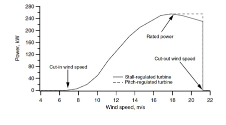
Figure 1: Wind turbine power curve [2]
Power curves are influenced by a wide range of variables, and the reference power curve might only be applicable to specific climatic or topographic regions. Power generation deviates from the values anticipated by a manufacturer's reference power curve, according to extensive research on power curve accuracy and the effects of complicated wind regimes on turbine performance [3,[4,[5]]. However, a novel idea is to examine the variation between proxy and actual generation.
Additionally, turbulence severity, wind shear, and terrain can cause deviations in power curves [3], [4]. Additionally, estimating the vertical wind speed and shear profile using the standard power law equations can be erroneous due to various meteorological events, such as the Low-Level Jet that occurs in the Great Plains/Midwest region [5]. Additionally complicating wind conditions are terrain and wake effects.
These same factors are anticipated to have an effect on the findings because this research will use manufacturer sales power curves. But in the context of monetary settlements,
Turbine performance is said to be influenced by deviations from the warranty (reference) power curve, which is also referred to as operational risk and partially accounted for in predicted operating losses (discussed further in Section 2.2).
2.1.1 Wind Speed Characterization and Measurement
As shown in Figure 2, of this Engineering assignments the wind speed at a location varies with time, and the Weibull distribution is frequently used to describe the long-term wind speed probability distribution. A time series of the site's measured wind speed is constructed to create this distribution. The two most common time series to employ are those with 10-minute average wind speeds and 1-hour average wind speeds. A probability distribution, such as the Weibull, can then be used to fit a histogram of the recorded wind speed.
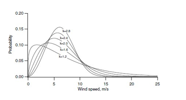
Figure 2: Weibull probability density function for U =6 m/s [2]
Scale and shape are the two parameters that make up the Weibull distribution. The distribution's mean and shape are determined by these characteristics.
The estimated energy output of a wind turbine is typically determined by integrating the product of the turbine power curve and the probability distribution of wind speed across all wind speeds. This results in a long-term forecast of the anticipated yearly(AEP) does not take into account seasonal fluctuations in wind speed. In other words, the amount of energy generated during any given season may be very different from what would be expected based on the long-term wind speed probability distribution [4]. There are variations that take place on shorter time frames in addition to seasonal variations.
Several methods, including a nacelle anemometer, a meteorological mast (met mast), or remote sensing equipment, can be used to measure and gather wind speed data. A combination of observations and models can also be used to estimate wind condition data, as is the case with MERRA (Modern Era-Retrospective Analysis for Research and Applications) (discussed further in Section 3). This study will look at proxy generation trends based on these many sources of wind speed data. An estimation of the wind speed without the rotor, which contains uncertainties, is necessary for nacelle anemometer wind speeds, which are obtained from anemometers positioned on the turbine nacelle's back. Met mast wind speeds originate from towers that are not necessarily near the turbines and, as a result of the impacts of the terrain, may have values that are different from the actual wind speed that a turbine experiences.
The use of MERRA reanalysis data, which are a synthesis of global wind observation data, is very recent for this application [6]. In addition to the previously mentioned uncertainty in data sources, wake effects from turbine-turbine interactions also contribute to the variability in wind speed readings. The accuracy of the proxy generation calculation will be examined in this analysis in relation to the effects of these various sources of wind speed.
2.1.3 Proxy Generation (PG)
Proxy generation is a production estimate that is based on idealised inflow circumstances. The following section [7] describes proxy generation.
NTF is the nacelle transfer function, and WSnacelle is the nacelle wind speed. PowerCurvewarranty is the power curve for the warranty (reference), and
Power performance losses, wake losses, lockage losses, and transmission losses inside the plant are all included in ExpectedOperationalLosses. The NTF ratio converts the nacelle wind speed to "free stream," and the corrected wind speed is utilised with the power curve to calculate energy. Both the NTF and the Power Curve are non-linear wind functions.
Even while it has only focused on performance in flat terrain, some study has started to look at the mistake in proxy creation [7]. With good measurement control, it has been demonstrated that the uncertainties from NTFs can range from 4 to 8%.
The final PG result is influenced by a wide range of distinct factors, each of which has the potential for mistake. The measurement of wind data is uncertain. Other potential causes include broken or malfunctioning equipment, improperly installed nacelle anemometers, and misaligned turbine controller settings. Project Met mast turbine pair data is used to construct the nacelle transfer function, which is subsequently applied to additional wind farm turbines without taking wake effects into consideration. Inflow angle, turbulence intensity, and mounting of the measuring arrangement are all important factors. The contract power curve from the manufacturer is the power curve employed in this equation, and the actual
Production will also differ (as discussed in section 2.1.1). Site calibration concerns exist in the projected operational losses, and proxy generation is known to understate these values [4]. The final proxy generation computation, which will be compared to the actual generated power, is affected by all of these causes of error.
2.2 Wind Energy Financial Models and Agreements
Since the beginning of the sector, wind energy finance models have undergone tremendous change, and current agreements are also undergoing modification [8]. Wind farms would sell their products directly into the electricity market if no financial arrangement were made. Since wind projects require stable revenue to be profitable, the emergence of standard PPAs was a response to the merchant structure's fluctuating cash flow effects. PPAs are continue to be phased out and replaced by swaps, hedges, and virtual power purchase agreements as a result of the lack of purchasers driving PPA costs low (discussed further in section 2.2.2 and section 2.2.3). The goal of our work on proxy generation is to enable financially sound agreements as the sector expands.
2.2.1 Power Purchase Agreements
Traditional PPAs are long-term, fixed-price agreements, often between a wind project and a utility or end customer of electricity, that last for 15-20 years [9]. There is a small pool of consumers (utilities and end users), but there are lots of producers (developers of wind projects), hence the costs for these kinds of agreements are low. As seen in Figure 3, fewer traditional PPAs are being created as a result of pricing and a dearth of purchasers. When wind projects are compelled to seek out alternate arrangements, the number of synthetic PPAs rises [10].
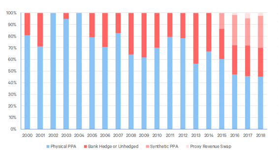
Figure 3: Since 2000, the amount of US wind capacity installed has been broken down into physical PPA or commercial structures [11].
With regard to the erratic and unpredictable nature of the wind, this financial structure is made simpler by charging a fixed fee per kilowatt hour in a PPA [12]. This, however, pushes wind projects to sell electricity at a lower, guaranteed price, which may result in less profit. Because typical PPAs are becoming less expensive, the industry is shifting toward alternative contracts that aim to take into account the intricacies of wind speed variability, boost revenue, and still safeguard wind projects from changes in energy prices [11].
2.2.2 Financial Hedging and Strategies
Cash flows for wind energy projects have been able to be stabilized through the use of financial agreements like hedges and virtual PPAs. According to their name, virtual PPAs never actually involve an exchange of electrons between the counterparty and the wind farm. Rather, both of the
Direct wholesale market transactions between a wind farm and counterparty result in a settlement between the two parties equal to the difference between the market and pre-set fixed price. Renewable Energy Credits (RECs) for the counterparty may also be an advantage of virtual PPAs [13]. In a bank hedging agreement, the wind farm commits to producing a specific amount of electricity, but the settlement sum varies according on the energy market price.
The payment arrangement for a virtual PPA between the hedge provider (company), electricity market (power pool and utility), and wind project (renewable energy system) is shown in Figure 4 below.
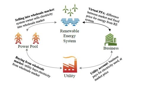
Figure 4 shows examples of digital PPA transactions [10]
The Actual Generated Quantity (AGQ) is frequently utilised in virtual PPAs to establish the fixed price of energy [7]. The AGQ represents how much energy the project actually produces. The hedge provider may experience problems if AGQ is used to settle price.
when the amount created is not what was anticipated. Operational risk resulting from clashing interests between the hedge provider and the wind farm is one element that could be problematic [14]. The counterparty wants to have no exposure to operational risk because AGQ is partially reliant on how well the wind farm is operated and maintained. The operational risk is eliminated for the hedge provider by using Proxy Generation (PG) as opposed to AGQ, which is based on measurable input rather than measured output [15]. Given a set of weather circumstances, PG estimates the amount of energy that the wind farm should produce, placing the operational risk on the wind farm, which is the entity in charge of the operation.
No matter how much electricity is produced, the wind farm is still liable for paying the settlement sum for bank hedges. Wind is a variable resource, yet a fixed amount of electricity must be delivered regardless, hence the wind project must assume the risk associated with the weather. This is lessened by proxy generation, which permits projected energy production to vary in accordance with the measured availability of the wind resource.
2.2.3 Financial Settlements with PG
In order to strengthen financial agreements for both sides, the accuracy of proxy generation will be increased. This will give hedging providers and wind farms a clearer idea of what the project should have produced. There is therefore a chance that wind readings will affect project revenue. Through two major financial settlements—the Proxy Generation virtual PPA (PG-vPPA) and the Proxy Revenue Swap—PG is now responsible for the financial health of wind project (PRS). Similar to virtual PPAs, PG-vPPAs function.
Regardless of the amount of energy used or the cost of electricity, PRS have a predetermined lump sum. This amount serves as a standard; if proxy revenue surpasses benchmark (lower than anticipated wind speeds or prices), project pays counterparty; if proxy revenue falls short of benchmark (lower than expected wind speeds or prices), counterparty pays project [16].
The advantage of PG is that it decouples operational risk from the counterparty [11], [7], allowing the party in charge of operations (the wind farm) to manage operational risk. As a result of the agreement's structure and flexibility in that it does not require a set amount of power to be produced, the wind farm is encouraged to run at maximum efficiency [11]. As the wind farm is no longer required to provide a specific amount of power, PG in the financial settlement also permits freedom on their part. The counterparty is in charge of weather risk, which is reduced by using PG-based financial agreements because they are better equipped to handle these weather variations [17]. Unlike earlier virtual PPAs and hedge agreements, these contracts provide protection for both parties.
When wind and price are unfavourably connected, there are some price concerns involved with employing PG estimations. As can be observed in Figure 5, ERCOT South exhibits a sharp increase in hub pricing at low generation levels, which are indicative of low wind speed. Due to the correlation between pricing and PG error, it is crucial to not only reduce total PG error but also comprehend underlying trends, particularly at interest wind speeds.
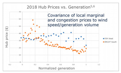
Figure 5: Hub Prices vs. Generation [7]
Figure 5 shows an instance that happened on a hot summer day in Texas when there was little wind and there was a huge demand for energy because of the massive power that A/C units used. The 10–12 February 2021 Texas hurricane was another startlingly expensive energy event, with the cost of energy reaching $9,000/MWh. The wind farm is still liable for the settlement if there is a sizable difference between proxy and actual generation during these pricing events. As a result, the financial performance of the wind farm may be significantly impacted by various proxy generation calculation techniques, which will be discussed more in Section 6.
CHAPTER 3
SITE OVERVIEW
3.1 Site Overview
North Texas is the location of the wind farm that was examined for this research, and Figure 3-1 depicts its layout. With a wintertime northerly component, the winds are primarily from the south. Take note of the 4 triangles designating met masts:
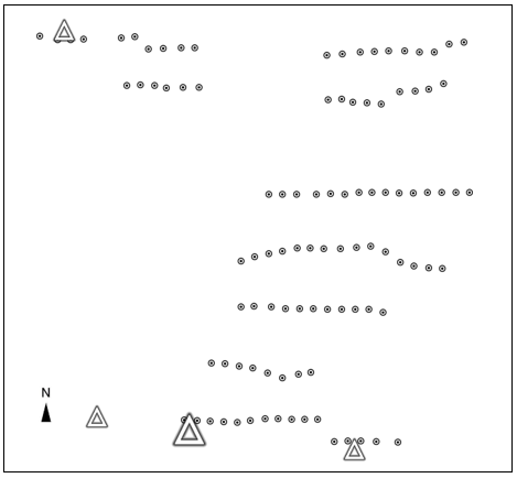
Figure 6: Turbine layout at project
3.2 Dataset
3.2.1 Turbine SCADA data
For all turbines from December 1, 2017, to November 30, 2018, 10-minute intervals of turbine SCADA data are supplied. This dataset includes the following variables: turbine power, nacelle wind speed, rotor position, operating status, temperature, and density corrected nacelle wind speed. A turbine OEM-applied nacelle transfer function, which is not site-specific, is used instead of a nacelle anemometer's raw wind speed data. The NTF approach enables the application of a further, site-specific NTF (discussed further in chapter 4).
3.2.2 Mast data
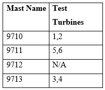
Three permanent and one temporary met masts were installed at the location. Masts 9710–9712 contain data from the SCADA system, while mast 9713 contains non–SCADA data from the Campbell Scientific data logger. The fourth one wasn't used in this investigation, and only three of them are linked with test turbines.
3.2.3 MERRA-2 Reanalysis data
The NASA Global Modeling and Assimilation Office's long-term global reanalysis effort is the Modern-Era Retrospective analysis for Research and Applications, Version 2 (MERRA-2) dataset. In the latitudinal direction, the spatial resolution is around 50 km. Data on the wind state are provided every hour at heights of 10 m and 50 m.
3.2.4 ERCOT Price data
The Electric Reliability Council of Texas (ERCOT) HB West hub provided the price dataset for this investigation in 15-minute intervals. During the analysis period, the highest price per MWh was $1406.43, and the lowest was -$18.40.
3.3 Data Filtering and Analysis
Filtering the raw data from the turbine and mast data was the initial phase, followed by building the framework to produce proxy generation figures. Python was used to complete this.
The following are the steps for data filtering:
1. Using the pairings in Table 2, combine the turbine and mast data using timestamps.
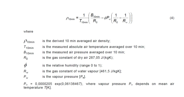
2. Determine the air density for every 10-minute data point. Due to the area's flat geography, a single density dataset that was based on data averaged between Masts 9710 and 9711 was used for the project. The following equation can be used to determine air density (taken from IEC 61400-12-2 9.1.1 Eq 4):
3. Determine the power curve's turbulence class (medium). For details, refer to the Appendix.
4.) Change the ERCOT pricing database's intervals from 15 to 10. For information, see Table 1.

CHAPTER 4
NACELLE TRANSFER FUNCTION (NTF) METHOD
4.1 Model Development
The NTF method determines the power production for each individual turbine by using measurements taken on-site from met masts and anemometers mounted on turbine nacelles. This data is then added together to determine the proxy generating value for the entire site. In order to account for the influence of the terrain on the wind speed measurement, this site-specific NTF offers an additional adjustment to the nacelle wind speed. These NTFs are created using Python programmes from met mast and turbine pair data. Following is a diagram of the turbine/mast coupling in Table 2:
Table 2: Mast/Turbine Coupling
The NTF approach involves the following procedures for generating proxy generation and proxy revenue values:
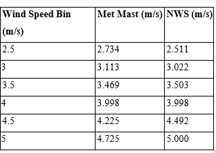
1. For valid data, compute Nacelle Transfer Functions (NTF). In this instance, the nacelle anemometer wind speed (NWS) and front-of-rotor, or "free stream," wind speed are related via a reference table (NTF), with the met mast serving as free stream. Data from a time period with both valid met mast and NWS accessible was chosen, and it was processed in accordance with the requirements of IEC Standard 61400-12-2. Utilizing only information from unrestricted direction sectors, subject to the restrictions listed in Appendix E. The data were divided into 0.5 m/s bins, and the ratio between the met mast and the NWS was determined for each bin [18]. Each mast/turbine pair's data was used to construct an NTF. These offer a conversion ratio to translate the wind speed observed at the test turbine's nacelle into the wind speed reported at the corresponding met mast. Table 2 provides a list of mast/turbine couples. There are seven NTFs in total, including the six mast/turbine pair NTFs and a site-wide NTF that uses the data from all mast/turbine pair NTFs averaged together. Seven different PG results are computed using them, and they will be contrasted in section 4.3.
The full NTFs are included in Table 3 along with an example NTF. The average wind speed for all wind speeds between 2.25 and 2.75 is contained in wind speed bin 2.5. The average wind speed at the met mast is known as Met Mast, while the average wind speed at the nacelle is known as NWS.
Table 3: NTF for Turbine 1
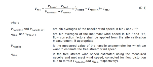
2. Utilizing linear interpolation, apply NTF to all reliable nacelle wind speeds from every turbine at the location. The following equation is employed (taken from IEC 61400-12-2 D.4 Eq D.1 [19]):
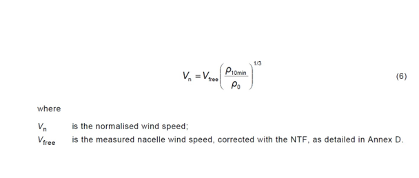
3. Adjust the free stream wind speed to the contract power curve's reference air density. The formula is as follows. (from IEC 61400-12-29.1.1 Eq 6):
4. Use linear interpolation to determine proxy generation by applying the power curve to normalized free stream wind speed. Now we'll have a proxy value of each turbine's generation. For further information on power curves, see Appendix A.
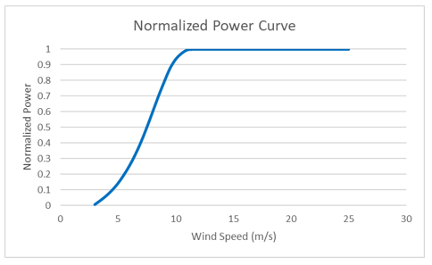
Figure 7: Manufacturer power curve
5. Sum turbine output at each time stamp to generate proxies over the entire site
6. Evaluate proxy generation revenue using price information:
???????????????????? ???????????????????????????? = ???????????????????????????????????????? (?????????) ∗ ???????????????????? ($ /?????????)
7. Repetition of steps 2 -6 with the remaining NTFs. There will be a set of PG results for each NTF, for a total of seven sets.
8. To analyze the effects of the site-specific correction, steps 3-6 are finished using the nacelle wind speed rather than the corrected free stream.
4.2 NTF Method Validation
The created NTFs were then compared to earlier research. Overall, the values appear to be consistent, demonstrating the validity of the methodologies employed here and the suitability of the NTF model for further investigation.
4.3 Error in NTF model
The NTF model depends on onsite measurements, which are costly, require upkeep, and require calibration. To accurately capture the front-of-rotor "free stream" to nacelle anemometer wind speed relationship, it is difficult to determine how many mast/turbine pairs are required. It was feasible to assess the potential range of results if various configurations were implemented by comparing the proxy generation results from all mast/turbine pairs. The nacelle anemometer wind speeds were employed in the calculation of an additional nacelle wind speed (NWS) proxy generation result without the addition of an NTF ratio. Analyzing the effects of on-site measurements and site-specific NTFs was possible. Results from six distinct test turbine NTFs, as well as a comparison with the NWS and site-wide NTF, are shown in
Figure 8. One is the slope of the red dashed line.
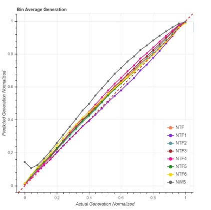
Figure 8: Bin Average Generation for all NTFs
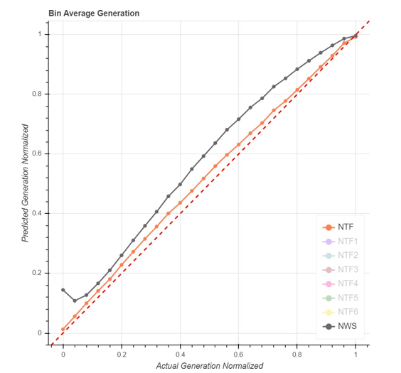
Figure 9: Bin Average Generation for site wide NTF and NWS
The distinction between the site-wide NTF and the NWS findings' bin average generation is depicted in Figure 9 above. The annualised proxy generation calculations in Table 4 reflect that the NWS results overpredict generation by a significant margin compared to the site-wide NTF. The influence of the site-specific NTF is clearly shown by this chart.
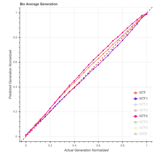
Figure 10: Bin Average Generation NTF method range
Along with the biggest and smallest NTF mast-turbine pair generating estimations, Figure 10 displays the site-wide NTF data. This illustrates the "working envelope" of the various mast-turbine pairs as well as the variety of possible outcomes in scenarios where there are less mast-turbine pairs at the location. Varying mast/turbine combinations will produce different NTF ratios as a result of the terrain's variation, which ultimately affects the wind project's financial performance.
The findings for the same mast and various turbine sets are shown in Figures 11 and 12 below. The largest variation between this type of pair is seen in Figure 11, illustrating how even with the same met tower, topography influences and other turbine variations may have an impact on NTF generation.
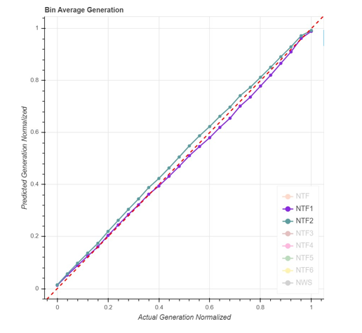
Figure 11: Bin Average Generation mast/turbine pair comparison 1
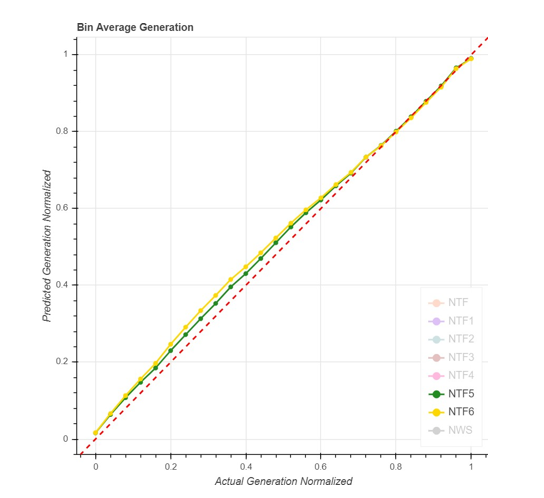
Figure 12: Bin Average Generation mast/turbine pair comparison 2
The outcomes of the NTF method's proxy production and revenue are shown in Tables 4 and 5. The site-wide average for the NTF comparison for proxy generation falls about in the middle of the range of errors, which vary from a 3% underestimate to a 10% underestimate. The range of the proxy revenue results is between a 9% and a 1% underestimation.
Compared to the outcomes with a site-specific NTF, the NWS model greatly overestimates both generation at 2% and revenue at 7%. This outcome illustrates how the site-specific NTF affects the precision of the production estimate. The nacelle anemometer and turbine OEM applied NTF do a poor job of capturing the impacts of terrain on wind speed.
Table 4: NTF Proxy Generation
Table 5: NTF Proxy Revenue
With the goal of investigating the effects of terrain and met mast distance on the accuracy of the PG estimate, Figure 13 below shows the distance between the test turbine/met mast with the error in PG and Proxy Revenue (PR). Given that the site's landscape consists of of flat farmland, it appeared logical that the discrepancies in the PG results would be more affected by the distance to the met mast. There isn't a clear causal link between the two, though, according to these findings.
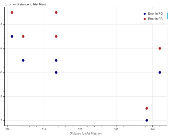
Figure 13: Distance to Met Mast vs Error
CHAPTER 5
REANALYSIS DATA METHOD
5.1 Model Development
The Reanalysis Data technique forecasts site-wide power production using a single wind speed and direction pair derived from the MERRA-2 database. In the absence of turbine SCADA or other site measurements, the financial agreement may be established by calculating proxy generation using reanalysis data.
A power matrix—a lookup table of wind speed and wind direction that calculates site-wide power—is generated using measured data from the turbine and mast. The met masts were used to establish wind speed and direction binning for the power matrix in order to take array and obstruction effects into account.
Table 6: Power Matrix Valid Sector Designations
The following are the stages to creating the power matrix:
1.) In order to calculate site-wide power, the power from each individual turbine was added at each timestamp where availability was more than 90%, and the associated met mast wind speed and direction were used.
2. To build the power matrix, the power was averaged over wind speed and wind direction. These manual edits were made:
a.) Based on the warranty power curve, power was taken to be zero at wind speeds below cut in.
b.) Unfilled bins were filled with the average site-wide rated power at wind speeds above the rated power up to the cutout wind speed.
Find the power matrix in Appendix D.
The following are the steps to generate proxy generation and proxy revenue figures using Python scripts and the Reanalysis Data method:
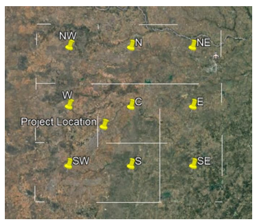
1.) From the database, MERRA-2 data for the nine grid locations closest to the wind farm were obtained. This investigation focused on the four closest to the project, denoted below by the letters W, C, SW, and S.
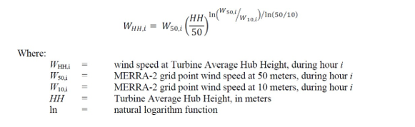
2.) To calculate hub height wind speed, a wind shear extrapolation model is utilised in conjunction with MERRA-10 m and MERRA-50 m wind speed information. The formula is as follows:
3.) To calculate the estimated project wind speed, four nearby MERRA-2 hub height wind speed sites are used (EPWS). Here is the equation that is used:
.png)
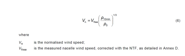
4.) The following equation normalises the EPWS to the site air density. (from IEC 12-2 9.1.1 Eq 6):
After that, using the wind speed information gathered at the met mast in the legal
sector, the normalised EPWS is rectified:
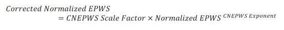
By fitting MERRA and each sites met mast wind speed exponentially, the CNEPWS Scale Factor and CNEPWS Exponent were determined. The exponents and scale factor from each of these were averaged. Results for the scale factor and exponent are shown in Table 7 below.
Table 7: CNEPWS Scale Factor and Exponent
As a weighted average of the wind vectors for each of the MERRA-2 grid points, the 50 m project wind direction was derived. Each wind vector's weight was determined by the inverse-square distance between the corresponding MERRA-2 grid points and the project site's geographic centre.
7.) The MERRA corrected hub height wind speed and the MERRA-50 m project wind direction are both subjected to the power matrix. The wind direction and wind speed at each timestamp were determined by linear interpolation to be closest to the value in the power matrix.
a. Error in reanalysis (MERRA-2) model
Three elements needed to be analysed to determine the MERRA-2 technique error:
1. Direct parameter comparison between onsite measurements and MERRA-2.
2. A comparison of proxy generation to look at flaws in the power matrix and outcomes after transformation through turbines.
3. A comparison of proxy revenue is used to assess the financial effects of the power matrix approach and any potential PG error amplification.
Figure 14 below is a scatter plot of MERRA-2 against wind speeds recorded at Met9711. It begins with the direct parameter comparison of onsite measurements vs. MERRA-2. Despite being site adjusted, it is evident that MERRA-2 estimations already have substantial differences from the site's real wind speeds (step 5 in Section 5.1). The comparisons between proxy revenue and proxy creation are covered in Chapter 6.
.png)
Figure 14: MERRA-2 vs Met 9711 Wind Speeds
CHAPTER 6
MODEL COMPARISONS
6.1 Proxy Generation and Revenue comparisons
The results of both the NTF method and the MERRA-2 method came from time series data collected from January 2018 to September 2018. By comparing results from the same time period, you can look at the financial effects of each estimate of power production during that time.
In Figure 15, you can see how real generation compares to MERRA-2 and the NTF method. It's clear right away that the NTF method is much closer to how generation really works. The NTF method has a much smaller error spread and a lower risk of a single event. The most important things are big differences between the proxy generation and the real generation, especially if they happen at the same time as a big price change. This is a lot more likely to happen with MERRA than with NTF.
Figure 16 shows how real income compares to MERRA-2 and the NTF method. The MERRA results show that errors are much more spread out, especially when revenues are higher.
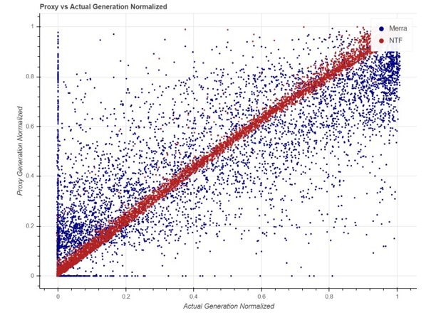
Figure 15: Proxy vs Actual Generation Scatter
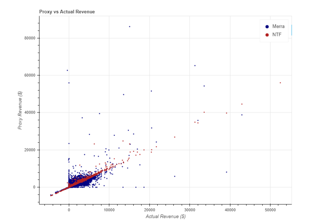
Figure 16: Proxy vs Actual Revenue Scatter
Error in generation and income are shown as a time series in Figure 17. Here, Error in Generation shows the same patterns as Figure 15. The error spread for MERRA is a lot bigger than that for NTF. When the error is big and the price of electricity is high, events tend to stand out more in the revenue time series.
During the time we looked into, there were two times that stood out. From March 8 to 10 and July 19 to 26, 2018, the error in MERRA-2 is always big, while the error in the NTF method is close to zero. After more research, it was found that none of the turbines at the site were working normally at these times. It is likely that the turbines were turned off for maintenance at these times. Taking these times out of the dataset didn't change the final results much, so they were kept.

Figure 17: Proxy – Actual Generation and Revenue Timeseries
Figure 18's two histograms are incorrect. No such source was found. Show the two approaches' different error spreads once more, highlighting how the MERRA-2 method's error range is substantially wider than the NTF method's.
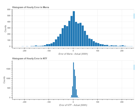
Figure 18: Error in PG Histogram
Below is an overview of statistics in Table 8. The mean error of 5.15 MWh is not yet representative, and the true value is slightly less because the operational efficiency losses have not yet been taken into account by the NTF technique in this case. Despite the fact that MERRA-2 mean error
It is evident from both the histograms and accompanying standard deviations that the error of the NTF method is much lower and is only marginally higher than that of the NTF approach.
Table 8: Summary Statics for Error in PG
Table 9: Summary Statics for Error in PR
The annualised generation and revenue of the two approaches are contrasted with the actual amounts in Table 10 below. The MERRA approach only has a mean error of 5% when generating proxies, but since the method overestimates project revenue by 7%, the proxy revenue demonstrates that the inaccuracy in generating proxies was poorly timed with the price of energy. In comparison, the NTF technique underpredicts project revenue by just 3% and its prediction diminishes from generation to revenue.
Table 10: PG and Actual Generation and Revenue Comparison
The annualized findings show that the percent error in PG for MERRA is in the same ballpark as the results from the NTF approach. However, shorter time frames need to be examined for the effects of a price excursion, which are further explored in the section below.
6.2 Time duration analysis
If the duration of these approaches is substantial, the error will probably have a greater effect. The settlement computation is unaffected if the model makes some over predictions and some under predictions, but evens out to zero error over the period of an hour. A price excursion event could occur and have an impact on the outcomes if the model "evens out" the inaccuracy over the course of several hours or days. As a result, we looked at how long it would take for the error to become equal.
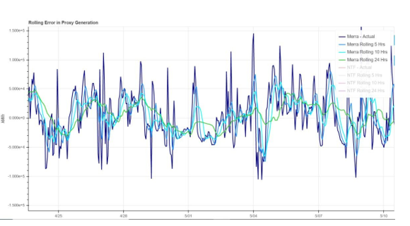
Figure 19: MERRA-2 Rolling Avg Error Generation
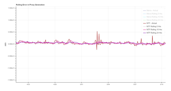
Figure 20: NTF Rolling Average Error Generation
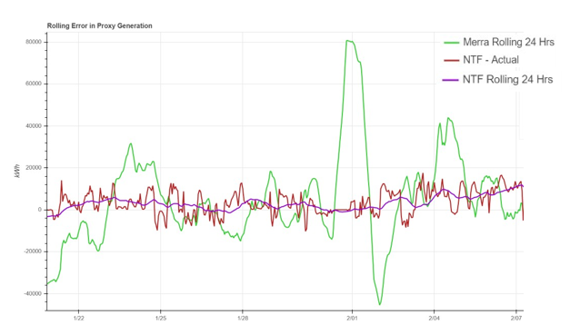
Figure 21: NTF vs MERRA Rolling Average Error in Generation
On a rolling average of 1, 5, 10, and 24 hours, Figures 19 and 20 above display the MERRA-2 and NTF error in generation, respectively. The NTF technique is balanced by rolling error significantly.
Even with a 24-hour rolling average, MERRA-2 still exhibits a significant magnitude of inaccuracy.
Comparing the NTF hourly and rolling average 24 hours to the MERRA-2 rolling average 24 hours is shown in Figure 21. The level of error between the two strategies differs significantly. For instance, a wind farm using the reanalysis method for their settlement would have to pay a much higher settlement than one using the NTF method if the significant green spike that appears in the MERRA-2 result at 01 February had actually occurred in Texas between February 10 and 12, 2021, when the price of energy was $9000 MWh. The primary focus of this work is on this kind of price excursion that correlates with significant errors in energy estimations. It is obvious that the NTF technique outperforms the MERRA-2 reanalysis method in proxy generation calculations by offering reduced price risk.
The rolling average errors in wind speed and proxy generation are shown in Figures 22 and 23, which provide additional analysis in the MERRA-2 approach to identify the error. On an hourly time scale, the MERRA-2 wind speed error is much worse than the onsite observations (see section 5.2), however when looking at the rolling average error up to 24 hours, it significantly decreases. As MERRA-2 is known to be less accurate at finer temporal scales, this is not surprising.
The same trends, however, are not visible when looking at the MERRA-2 proxy generation's rolling average error. Figure 23 displays the rolling error in PG over various longer time periods up to one month, and the MERRA-2 values still have a wider range and more uneven distribution of error than the NTF approach. This suggests that a significant portion of the reanalysis data method's errors come from the power matrix.
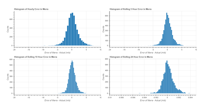
Figure 22: MERRA-2 Wind Speed Rolling Average Histograms
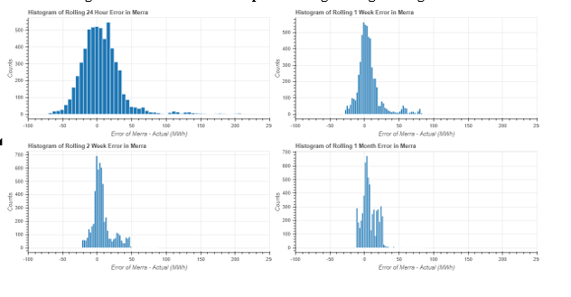
Figure 23: MERRA-2 PG Rolling Average Histograms
An error matrix for MERRA-2 is shown in Figure 24 below. This investigation was done to see if there were any parts of the power matrix that were primarily to blame for the MERRA-2 error. Instead, all of the places with significant inaccuracy were concentrated near where the majority of the information was. Additionally, cells with large over- and underestimates were all situated close to one another. Future research should focus on this because it appears to show that the error is rather random (discussed further in Section 7.2.1).
Figure 24: MERRA-2 Error Matrix
CHAPTER 7
CONCLUSIONS AND FUTURE WORK
7.1 Concluding Remarks
The mast/turbine pair configuration at the site is proven to affect the NTF method results, which eventually affects the project proxy revenue. One of the risk factors in the NTF technique is the number of met masts and mast/turbine pairings at the site. In comparison to using only the nacelle wind speed with the OEM corrected NTF, using met masts and a site-specific NTF considerably improves the accuracy of both wind turbine power forecast and proxy revenue. The results of this case study demonstrate that the reanalysis data method, which attempts to estimate the site-wide proxy generation using a single wind direction and wind speed, is a subpar estimation technique.
Overall, employing local wind condition observations for turbine power prediction has significant advantages. The NTF approach manages price excursion risk significantly better than MERRA-2. The unfavorable association between wind and pricing was one of the initial driving forces behind this initiative. The events in Texas in February 2021 were an extreme example illustrating a conceivable scenario in which various power projection systems may have a significant impact on the financial settlement for a wind farm [20].
The financial settlement may be determined using proxy generation results from MERRA-2 data if turbine SCADA or other on-site measurements are not available.
The cost repercussions of that decision are demonstrated by contrasting the NTF technique and MERRA-2 results. The wind farm may experience serious financial consequences if a severe price event coincides with a financial settlement determined using MERRA-2.
7.2.2 Additional projects
This case study was performed on a wind site in north Texas, with relatively simple terrain. This analysis should be performed on data from other wind projects, as well as those in more complex terrain. Financial settlements using the PG values from both NTF and reanalysis data methods are already in place without an understanding of the financial implication of either method. Better understanding of the impacts of each method across varied terrain should be explored.
7.2.3 Applications in other agreements
Other uses for the creation of two distinct models to forecast site-wide electricity generation exist in addition to wind farm financial agreements. Now, settlement and curtailment agreements as well as contractual guarantees can be analysed using the methodologies developed here.
REFERENCES


- MGT502 Business Communication 1 B Report
- MKG203 Digital Marketing Communication Assignment
- BUS6001 Business Strategy Management Assignment
- MIS602 IT Report
- ICT102 Networking Report 3
- COIT20251 Knowledge Audit for Business Analysis Report
- ITECH1103 Big Data and Analytics Assignment
- COIT20246 Networking and Cyber Security Assignment
- GDECE101 Early Childhood and Education Essay
- MGMT6009 Managing People and Teams Report 1
- Marketing Fundamental Report
- HCT343 Research Methods and Data Analysis in Healthcare Assignment
- MGT602 Business Decision Analytics Research Report 3
- Auditing Coursework Assignment
- MIS607 Mitigation Plan for Threat Report
- ECO500 Economics for Business Assignment
- NUR1203 Cultural Safety and professional Practice Assignment
- MBIS4010 Professional Practice in Information Systems Essay
- STAT6003 Statistics for Financial Decisions Assignment
- DATA4500 Social Media Analytics Report 3


.png)
~5.png)
.png)
~1.png)


.png)